Creating A Calculated Measure Cube - IOGALFF

(Firstly, this is information relates only to OLAP 10gR2. There are a number of changes within OLAP11gR1 and the following scenario has not been tested with 11g)

When you venture into most supermarkets today, somewhere on one of the many isles there will be a BOGOF – buy one get one free. Well how about an OLAP offer: “IOGALFF” – install one get at least fourteen free. I admit it is not quite as catchy as the original, but the benefits are huge and it has the result of making life so much easier.

One of the more interesting challenges of using Analytic Workspace Manager (and also OWB) relates to managing all the calculated measures within a cube. Every measure should really be accompanied by a standard set of calculated measures such as:

• Current Period
• Last Year
• Last Year %
• Prior Period
• Prior Period %
• Year to Date
• Year to Date Last Year
• Year to Date Last Year %
• Quarter to Date
• Quarter to Date Last Year
• Quarter to Date Last Year %
• 3-Month Moving Average
• 6-Month Moving Average
• 12-Month Moving Average
• Dimension “A” Share of All Members
• Dimension “A” Share of Parent

Its is the addition of these types of measures that adds real value to the your BI application. As I have stated many times before: business users are not interested in looking at data from base measures, typically they are more interested in trends based on the prior period or prior year, share of revenue, moving averages and so on. This adds a lot of work for the cube designer as they need to add at least 14 calculated measures for each base measure as well as two additional calculated share measures for each dimension associated with each cube.

Which adds up to a lot of measures and manually creating all these measure is likely to take a considerable amount of time. If we take the command schema sample that is shipped with BI10g, this contains 5 base measures (costs, quantity, revenue, margin, price) with 4 dimensions (channel, geography, product, time), which translates to

5 * 14 calculated measures
+
5 * 3 (dimensions - channel, geography, product) * 2 calculated share measures

= 100 calculated measures.

As I said, it is very easy to generate a lot of calculated measures.


So is there a more intelligent way of managing calculated measures? What is the quickest way to add all these additional calculations to a cube? One way is to use the Excel Accelerator to add the calculated measures to your AW. It is relatively easy to use and allows you to use normal Excel tools such as cut & paste to quickly create all the calculations you could ever need. You can download the Excel Accelerator from the OLAP OTN Home Page, or by clicking here. Look for these links:

Creating OLAP Calculations using Excel
Creating OLAP Calculations using Exce Readme

During a recent POC, we used a more interesting approach that takes the use of customer calculations to a new level. In many ways this goes back to the various techniques we used when creating Express databases for use with Sales Analyzer to make life easier for both administrators and users. The approach is quite simple – use and additional dimension to define the type of calculation you want to execute and link this to a DML program to return the required results. The list of calculated measures listed above are converted into dimension members, which provides another way to slice, dice and pivot the data. As you can see here, the dimension member that identifies the type of calculation is in the row edge with the measure in the column edge. In this way, only one calculation is required which is used across all the available measures.



What this means is: by installing one simple (well, everything is relative) calculated measure you can get upto fourteen additional calculations for free. Hence the acronym “IOGALFF” – install one get at least fourteen free.

How is all this managed? There are five basic steps to creating this type of reporting solution:

1. Create a new dimension to control the types of calculations returned
2. Add some additional attributes to the time dimension to help manage some of the time series arguments for specific calculations
3. Create an OLAP DML program to return the data
4. Create a new cube that includes the new calculation type dimension and add a calculated measure that calls the OLAP DML program to return the required data
   
5. Create a SQL View over the cube

Step 1 – Creating the new Time View dimension

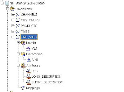
I have called the dimension containing the list of calculated members, Time View (mainly because the majority of the calculations are time based but may be a better name would be "measure view" ?). The Time View dimension has one level and one hierarchy with three attributes:

• Long Label
• Short Label
• Default sort order

The source data looks like this:



With the source table definition as follows:

CREATE TABLE TIME_VIEW
(TIME_VIEW_ID VARCHAR2(2 BYTE),
TIME_VIEW_DESC VARCHAR2(35 BYTE),
SORT_ORDER NUMBER(*,0));

And the view definition as follows:

CREATE OR REPLACE FORCE VIEW VW_TIME_VIEW AS
SELECT
TIME_VIEW_ID
, TIME_VIEW_DESC
, SORT_ORDER
FROM TIME_VIEW
ORDER BY SORT_ORDER;

To populate the base table the following commands are used:

INSERT INTO TIME_VIEW VALUES ('1', 'Current Period', '1')
INSERT INTO TIME_VIEW VALUES ('2', 'Last Year', '2')
INSERT INTO TIME_VIEW VALUES ('3', 'Last Year %', '3')
INSERT INTO TIME_VIEW VALUES ('4', 'Prior Period', '4')
INSERT INTO TIME_VIEW VALUES ('5', 'Prior Period %', '5')
INSERT INTO TIME_VIEW VALUES ('6', 'Year To Date', '6')
INSERT INTO TIME_VIEW VALUES ('7', 'Year To Date Last Year', '7')
INSERT INTO TIME_VIEW VALUES ('8', 'Year To Date Last Year %', '8')
INSERT INTO TIME_VIEW VALUES ('9', 'Quarter To Date', '9')
INSERT INTO TIME_VIEW VALUES ('10', 'Quarter To Date Last Year', '10')
INSERT INTO TIME_VIEW VALUES ('11', 'Quarter To Date Last Year %', '11')
INSERT INTO TIME_VIEW VALUES ('12', '3-Month Moving Average', '12')
INSERT INTO TIME_VIEW VALUES ('13', '6-Month Moving Average', '13')
INSERT INTO TIME_VIEW VALUES ('14', '12-Month Moving Average', '14')

After this, the next set of values depends on the dimensions within your data model. For my model, I have three additional dimensions that I want to analyze: Channel, Product and Customer. For each of these dimensions I want to see the % share of each member in relation to the value for all members (i.e. the top level) and the shared based on the parent value. To enable these calculations I add the following lines to the TIME_VIEW table:

INSERT INTO TIME_VIEW VALUES ('15', ' Product Share of All Products', '15')
INSERT INTO TIME_VIEW VALUES ('16', ' Product Share of Parent', '16')
INSERT INTO TIME_VIEW VALUES ('17', ' Channel Share of All Channels', '17')
INSERT INTO TIME_VIEW VALUES ('18', ' Channel Share of Parent', '18')
INSERT INTO TIME_VIEW VALUES ('19', ' Customer Share of All Customers', '19')
INSERT INTO TIME_VIEW VALUES ('20', ' Customer Share of Parent', '20')

(Obviously, these additional share calculations are not really related to time, so using the name Time View is sort of confusing and in hindsight the term Measure View would have been a better name for the dimension). Once the table has been defined, it can be mapped in AWM to create the dimension mapping (in this case I am using a view over the source



The last part of this step is to then load the members into the dimension using the dimension data load wizard or via the SQL command line using a load script. The result should look like this when you view the members using the Dimension Data Viewer:



As can be seen here, there are fourteen base calculations that can be applied to any model, plus the additional share calculations that are based on the dimensions within the source cube. Hence the title “IOGALFF” – install one get fourteen free. In reality it is more like: install one and as many calculations as you like or need, but that translates to “IOGASMAYNORL” which does not really role off the tongue.

Step 2 – Updating the Time Dimension with new Attributes.

To make the program that delivers all these calculated measures as simple as possible a number of attributes are added to the time dimension:

• Lag Prior Year
• At the Year level this equates to 1
• At the Quarter level this equates to 4
• At the Month level this equates to 12
• At the Day level it is the number of days in the year (365 or 366)
• Parent Quarter
• This is the quarter for each time period and used as the reset trigger for the cumulative totals
• Parent Year
• This is the year for each time period and used as the reset trigger for the cumulative totals

The information for the two parent attributes is taken from existing columns within the source data since this information already exists and the Lag Prior Year is a simple hard-coded value apart from the day level where the timespan value for the year is used to cope with leap years. Therefore, all the information for these three attributes should be readily available within your source data, especially if you are using the OWB Time Wizard to create your time dimension. Obviously using a view over the source table for the mapping within AWM makes adding this information relatively trivial.

Step 3 – Create the OLAP DML Calculation Program.

The new OLAP DML program, called TIME_VIEW_PRG (again feel free to change the name of program if you want), takes two arguments:

• The cube.measure_name for the base measure, in this case SALES_M1, which is the Revenue measure in the SALES cube.
• The identifier for the calculated measure within the REPORT_CUBE cube, which in this case is M1_PRG (this is explained in more detail in the next section)
  

The program code is as follows, which for those of you familiar with OLAP DML will find relatively easy to understand:

DEFINE TIME_VIEW_PRG PROGRAM DECIMAL
argument T_MEASURE text " Full measure name including cube name
argument T_MEASURE_ID text " Measure name

variable T_FORM text " Name of the formula
variable T_TIME_VIEW text " Value of TIME_VIEW dimension
variable D_RETURN decimal " Return value

trap on ALLDONE noprint

T_TIME_VIEW = TIME_VIEW
T_FORM = joinchars('REPORT_CUBE_', T_MEASURE_ID)

switch T_TIME_VIEW
do
case 'VL1_1':
D_RETURN = &T_MEASURE
break
case 'VL1_2': "LY
D_RETURN = lag(&T_FORM(TIME_VIEW 'VL1_1'), TIMES_LAG_PRIOR_YEAR, TIMES, LEVELREL TIMES_LEVELREL)
break
case 'VL1_3': "LY%
D_RETURN = lagpct(&T_FORM(TIME_VIEW 'VL1_1'), TIMES_LAG_PRIOR_YEAR, TIMES, LEVELREL TIMES_LEVELREL)
break
case 'VL1_4': "PP
D_RETURN = lag(&T_FORM(TIME_VIEW 'VL1_1'), 1, TIMES, LEVELREL TIMES_LEVELREL)
break
case 'VL1_5': "PP%
D_RETURN = lagpct(&T_FORM(TIME_VIEW 'VL1_1'), 1, TIMES, LEVELREL TIMES_LEVELREL)
break
case 'VL1_6': "YTD
if TIMES_LEVELREL EQ 'YEAR'
then D_RETURN = &T_FORM(TIME_VIEW 'VL1_1')
else D_RETURN = cumsum(&T_FORM(TIME_VIEW 'VL1_1'), TIMES, TIMES_PARENT_YEAR)
break
case 'VL1_7': "YTD LY
if TIMES_LEVELREL EQ 'YEAR'
then D_RETURN = lag(&T_FORM(TIME_VIEW 'VL1_1'), TIMES_LAG_PRIOR_YEAR, TIMES, LEVELREL TIMES_LEVELREL)
else D_RETURN = cumsum(lag(&T_FORM(TIME_VIEW 'VL1_1'), TIMES_LAG_PRIOR_YEAR, TIMES, LEVELREL TIMES_LEVELREL), TIMES, TIMES_PARENT_YEAR)
break
case 'VL1_8': "YTD LY%
D_RETURN = (&T_FORM(TIME_VIEW 'VL1_6')-cumsum(lag(&T_FORM(TIME_VIEW 'VL1_1'), TIMES_LAG_PRIOR_YEAR, TIMES, LEVELREL TIMES_LEVELREL), TIMES, TIMES_PARENT_YEAR))/cumsum(lag(&T_FORM(TIME_VIEW 'VL1_1'), TIMES_LAG_PRIOR_YEAR, TIMES, LEVELREL TIMES_LEVELREL), TIMES, TIMES_PARENT_YEAR)
break
case 'VL1_9': "QTD
if TIMES_LEVELREL EQ 'YEAR'
then D_RETURN = NA
else if TIMES_LEVELREL EQ 'QUARTER'
then D_RETURN = &T_FORM(TIME_VIEW 'VL1_1')
else if TIMES_LEVELREL EQ 'MONTH'
then D_RETURN = cumsum(&T_FORM(TIME_VIEW 'VL1_1'), TIMES, TIMES_PARENT_QUARTER)
else if TIMES_LEVELREL EQ 'DAY'
then D_RETURN = cumsum(&T_FORM(TIME_VIEW 'VL1_1'), TIMES, TIMES_PARENT_QUARTER)
else D_RETURN = NA
break
case 'VL1_10': "QTD LY
if TIMES_LEVELREL EQ 'YEAR'
then D_RETURN = NA
else if TIMES_LEVELREL EQ 'QUARTER'
then D_RETURN = cumsum(lag(&T_FORM(TIME_VIEW 'VL1_1'), TIMES_LAG_PRIOR_YEAR, TIMES, LEVELREL TIMES_LEVELREL), TIMES, TIMES_PARENT_QUARTER)
else if TIMES_LEVELREL EQ 'MONTH'
then D_RETURN = cumsum(lag(&T_FORM(TIME_VIEW 'VL1_1'), TIMES_LAG_PRIOR_YEAR, TIMES, LEVELREL TIMES_LEVELREL), TIMES, TIMES_PARENT_QUARTER)
else if TIMES_LEVELREL EQ 'DAY'
then D_RETURN = cumsum(lag(&T_FORM(TIME_VIEW 'VL1_1'), TIMES_LAG_PRIOR_YEAR, TIMES, LEVELREL TIMES_LEVELREL), TIMES, TIMES_PARENT_QUARTER)
break
case 'VL1_11': "QTD LY%
if TIMES_LEVELREL EQ 'YEAR'
then D_RETURN = NA
else if TIMES_LEVELREL EQ 'QUARTER'
then D_RETURN = (&T_FORM(TIME_VIEW 'VL1_9')-cumsum(lag(&T_FORM(TIME_VIEW 'VL1_1'), TIMES_LAG_PRIOR_YEAR, TIMES, LEVELREL TIMES_LEVELREL), TIMES, TIMES_PARENT_QUARTER))/cumsum(lag(&T_FORM(TIME_VIEW 'VL1_1'), TIMES_LAG_PRIOR_YEAR, TIMES, LEVELREL TIMES_LEVELREL), TIMES, TIMES_PARENT_QUARTER)
else if TIMES_LEVELREL EQ 'MONTH'
then D_RETURN = (&T_FORM(TIME_VIEW 'VL1_9')-cumsum(lag(&T_FORM(TIME_VIEW 'VL1_1'), TIMES_LAG_PRIOR_YEAR, TIMES, LEVELREL TIMES_LEVELREL), TIMES, TIMES_PARENT_QUARTER))/cumsum(lag(&T_FORM(TIME_VIEW 'VL1_1'), TIMES_LAG_PRIOR_YEAR, TIMES, LEVELREL TIMES_LEVELREL), TIMES, TIMES_PARENT_QUARTER)
else if TIMES_LEVELREL EQ 'DAY'
then D_RETURN = (&T_FORM(TIME_VIEW 'VL1_9')-cumsum(lag(&T_FORM(TIME_VIEW 'VL1_1'), TIMES_LAG_PRIOR_YEAR, TIMES, LEVELREL TIMES_LEVELREL), TIMES, TIMES_PARENT_QUARTER))/cumsum(lag(&T_FORM(TIME_VIEW 'VL1_1'), TIMES_LAG_PRIOR_YEAR, TIMES, LEVELREL TIMES_LEVELREL), TIMES, TIMES_PARENT_QUARTER)
break
case 'VL1_12': "3MMA
if TIMES_LEVELREL eq 'MONTH'
then D_RETURN = MOVINGAVERAGE(&T_FORM(TIME_VIEW 'VL1_1'), -2, 0, 1, TIMES, LEVELREL TIMES_LEVELREL)
else D_RETURN = NA
break
case 'VL1_13': "6MMA
if TIMES_LEVELREL eq 'MONTH'
then D_RETURN = MOVINGAVERAGE(&T_FORM(TIME_VIEW 'VL1_1'), -5, 0, 1, TIMES, LEVELREL TIMES_LEVELREL)
else D_RETURN = NA
break
case 'VL1_14': "12MMA
if TIMES_LEVELREL eq 'MONTH'
then D_RETURN = MOVINGAVERAGE(&T_FORM(TIME_VIEW 'VL1_1'), -11, 0, 1, TIMES, LEVELREL TIMES_LEVELREL)
else D_RETURN = NA
break
case 'VL1_15': "Product Share of All Products
D_RETURN = &T_FORM(TIME_VIEW 'VL1_1')/&T_FORM(TIME_VIEW 'VL1_1', PRODUCTS limit(PRODUCTS to TOPANCESTORS using PRODUCTS_PARENTREL)
break
case 'VL1_16': "Product Share of Parent
D_RETURN = &T_FORM(TIME_VIEW 'VL1_1')/&T_FORM(TIME_VIEW 'VL1_1', PRODUCTS PRODUCTS_PARENTREL)
break
case 'VL1_17': "Customers Share of All Customers
D_RETURN = &T_FORM(TIME_VIEW 'VL1_1')/&T_FORM(TIME_VIEW 'VL1_1', CUSTOMERS limit(CUSTOMERS to TOPANCESTORS using CUSTOMERS_PARENTREL)
break
case 'VL1_18': "Customers Share of Parent
D_RETURN = &T_FORM(TIME_VIEW 'VL1_1')/&T_FORM(TIME_VIEW 'VL1_1', CUSTOMERS CUSTOMERS_PARENTREL)
break
case 'VL1_19': "Channels Share of All Channels
D_RETURN = &T_FORM(TIME_VIEW 'VL1_1')/&T_FORM(TIME_VIEW 'VL1_1', CHANNELS limit(CHANNELS to TOPANCESTORS using CHANNELS_PARENTREL)
break
case 'VL1_20': "Channels Share of Parent
D_RETURN = &T_FORM(TIME_VIEW 'VL1_1')/&T_FORM(TIME_VIEW 'VL1_1', CHANNELS CHANNELS_PARENTREL)
break
doend


ALLDONE:
return D_RETURN
END

In simple terms, the program checks to see which member of the dimension TIME_VIEW is being requested and then executes the correct OLAP function to return the required data. At the moment this has only been tested on a Julian calendar hierarchy but I am doing some more testing over the next few weeks for other types of hierarchies. Some of the measures are dependant on the level within the Time dimension, so you may need to change references to specific level names etc if you want to reuse this program code. For example:

if TIMES_LEVELREL EQ 'YEAR'

My time dimension has levels; Year, Quarter, Month, and Day. In some cases it is necessary to change the processing depending the level, for example:

if TIMES_LEVELREL EQ 'YEAR'
then D_RETURN = NA
else if TIMES_LEVELREL EQ 'QUARTER'
then D_RETURN = &T_FORM(TIME_VIEW 'VL1_1')
else if TIMES_LEVELREL EQ 'MONTH'
then D_RETURN = cumsum(&T_FORM(TIME_VIEW 'VL1_1'), TIMES, TIMES_PARENT_QUARTER)
else if TIMES_LEVELREL EQ 'DAY'
then D_RETURN = cumsum(&T_FORM(TIME_VIEW 'VL1_1'), TIMES, TIMES_PARENT_QUARTER)
else D_RETURN = NA


In this code extract you can see the reference to one of the additional time attributes we added in the previous step, PARENT_QUARTER that is used by the program. All the references within the program are based on Standard Form naming conventions. Therefore, the full standard name for this attribute is TIMES_PARENT_QUARTER since the dimension is called TIMES and the attribute is called PARENT_QUARTER.

For simplicity I created the program in the AW containing the cubes, which is not exactly ideal because if you delete the AW to rebuild it you will lose the program code. Alternatively, you can just create a new AW and add the program to the new AW then modify the ONTTACH program in your data AW to automatically attach the program AW.

Calculations for dimension members VL_15 to VL_20 are provided as examples and would need to be changed to match the dimensions within your own AWs. For each dimension you will need to create two new dimension members within the TIME_VIEW dimension to return the following share calculations:

• Share of based on the top level total, i.e. All Members
• Share based on parent.

As the code uses Standard form notation the only thing you should need to change is code highlighted in bold and replace the phrase “Channels” with your own dimension name:

case 'VL1_19': "Channels Share of All Channels
D_RETURN = &T_FORM(TIME_VIEW 'VL1_1')/&T_FORM(TIME_VIEW 'VL1_1', CHANNELS limit(CHANNELS to TOPANCESTORS using CHANNELS_PARENTREL)
break
case 'VL1_20': "Channels Share of Parent
D_RETURN = &T_FORM(TIME_VIEW 'VL1_1')/&T_FORM(TIME_VIEW 'VL1_1', CHANNELS CHANNELS_PARENTREL)
break


Step 4 – Creating the New Cube.

In my demo schema I have a cube called SALES and it contains two measures: Revenue (called M1) and Quantity (called M2). The dimensionality for this cube is Time, Channel Product, and Customer.

To provide all the time series and comparative calculations I create a new cube that has the same dimensionality as the SALES cube, with one additional dimension. In this cube the Time View dimension is also used. This reporting cube contains no stored measures, but it does contain custom calculated measures for each measure in the SALES cube, however, each calculated measure will return 14 additional time calculations and 6 share calculations to support the base measure controlled by the dimension TIME_VIEW.



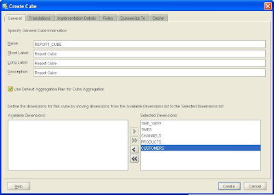
The implementation for the cube is largely irrelevant since no stored measures will be present within the cube, only calculated measures. Therefore, you can if you want either accept the default settings or de-select all the various options.



To add the calculated measures to the cube requires the use of a custom measure XML template. To create a calculated measure to support the measure “Revenue” from the SALES cube you will need to create a custom calculation either using an XML template (email me I can send you a blank template) or use the Excel Calculation Utility that can be downloaded from the OLAP Home Page on OTN to install the two custom calculations.

Once you have added these calculated measures to the REPORT_CUBE, the tree in AWM should look like this:



By selecting each of the calculated measures, the details of each calculation will be displayed within the right-hand panel of AWM. For the first calculated measure linked the Revenue measure in the Sales cube the panel looks like this:



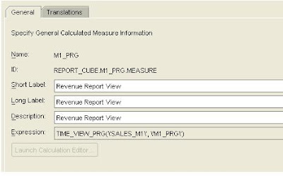
For the second calculated measure linked the Quantity measure in the Sales cube the panel looks like this:



The key part is the line showing the “Expression” (in the XML Template this is the attribute ExpressionText), this defines the call to an OLAP DML program called TIME_VIEW_PRG passing the two required arguments of

ExpressionText="TIME_VIEW_PRG('SALES_M1', 'M1_PRG')”

• The cube.measure_name for the base measure, in this case SALES_M1, which is the Revenue measure in the SALES cube.
• The identifier for the calculated measure within the REPORT_CUBE cube.

At this point you may or may not have the correct formula/expression text. When you load calculations via the XML interface OLAP tries to be a bit too clever and it attempts to convert any physical name it can match with the equivalent standard form name. In most cases this is fine, but in this case we need to refer directly to the physical objects. Modifying the expressions is relatively easy if you follow these steps. Using AWM, open the OLAP Worksheet and then:

1. CNS REPORT_CUBE_M1_PRG
2. EQ TIME_VIEW_PRG('SALES_M1', 'M1_PRG')
3. UPDATE
4. COMMIT
5. CNS REPORT_CUBE_M2_PRG
6. EQ TIME_VIEW_PRG('SALES_M2', 'M2_PRG')
7. UPDATE
8. COMMIT

If want to do this via the PL/SQL interface then you can do something like this:

EXEC DBMS_AW.EXECUTE('AW ATTACH AW_NAME RW FIRST')
EXEC DBMS_AW.EXECUTE('CNS REPORT_CUBE_M1_PRG')
EXEC DBMS_AW.EXECUTE('EQ TIME_VIEW_PRG(''SALES_M1'', ''M1_PRG'')')
EXEC DBMS_AW.EXECUTE('UPDATE')
EXEC DBMS_AW.EXECUTE('COMMIT')
EXEC DBMS_AW.EXECUTE('CNS REPORT_CUBE_M2_PRG')
EXEC DBMS_AW.EXECUTE('EQ TIME_VIEW_PRG(''SALES_M2'', ''M2_PRG'')')
EXEC DBMS_AW.EXECUTE('UPDATE')
EXEC DBMS_AW.EXECUTE('COMMIT')
EXEC DBMS_AW.EXECUTE('AW DETACH AW_NAME')


Step 4a – Viewing the Data.

Once the calculated measures have been added to the new cube, REPORT_CUBE, the AWM Data Viewer can be launched to check the results:



In the Query Wizard both sets of measures (stored measures and the new calculated measures) are both available for selection. To see the new calculations that are now available we can select both of the Report View measures as shown here.

Once the measures have been selected, the dimension selector will allow us to pick the calculations we want to display from the list of twenty (there are fourteen base calculations that can be applied to any model, plus the additional share calculations that are based on the dimensions within the source cube, in this case six additional share calculations, making twenty calculated measures in total).



The Dimension Viewer shows all the available calculations for this demo schema and the final report is shown below.




Step 5 – Making the Data Available via SQL.
Is there any real point to this post except to show how clever Oracle OLAP can be? In opinion yes, since this technique can be extremely useful when you need to make an OLAP cube visible to SQL based tools. Analytic Workspace Manager 10g has an relational view generator that is available as a plugin and this makes generating the SQL views to support your OLAP cubes a very quick and easy process. But there we know users don’t just want base measures they want lots and lots of calculations as well. When the time comes to create SQL views as the limit on the number of columns within a view is 1000. This may have been increased in 10g/11g, but even so, navigating a cube with that many columns is not easy.

The OLAP View Generator plugin for AWM10gR2 can be downloaded from here, and the associated readme is here.

Using this model, the calculations simply resolve to another dimension, which translates to one additional column in the view as opposed to, at least, 14 additional columns per source measure and in this case 20 additional columns per source measure. Therefore, this approach makes exposing the cube much easier to manage as can be seen here:



As we can see here, all the calculations are contained within the dimension Time View, which simply gets exposed like any other dimension.

Eh voila, install one measure and you can automatically generate fourteen or more additional measures which are guaranteed to bring a smile to the face of any business user.

OLAP Option Wiki Update

The OLAP Blog team has been adding lots of new content to the Oracle OLAP Option Wiki site. To link to the Wiki click here. We have added both general and techie/DBA focused information. Don't forget the Wiki is open to contributions from everyone within the Oracle community: customers, partners and oracle employees. To join the Oracle Wiki community simply click here, or go to http://wiki.oracle.com/accountnew. Registration is free.

This is what we currently have on the Wiki for the OLAP Option:

General Information
Background and History - of the OLAP Option. This covers the key milestones in the development of Express and its evolution into the the OLAP Option.

Getting Started with Oracle OLAP - This is a series of shortcuts to get you up and running with the OLAP Option as quickly as possible. We have included additional reading material and links to all the relevant documentation.

Terminology - Covers the key concepts and terms used when working with multidimensional data and more specifically the OLAP Option. There are still some blank pages but we are slowly making progress.

Versions - This page provides the key features for each version, from the latest version of the OLAP Option (11g Release 1) all the way back to Express Server 4.8. The Express server product line does go back much further (I started with PCX2.5, I think) but there is no documentation to consult to extract a list of features. If anyone can fill in the missing products please feel free to add the content.

Oracle OLAP Newsletter - Links to the current newsletter and archive copies. We have extracted the main headlines from each newsletter to make searching for a specific article a little easier.

For DBAs and Techies
Script Samples - A complete library of 29 scripts to help DBAs and developers manage the OLAP option.

Oracle OLAP How To - The purpose of this page is to cover basic principles and recommendations around generic tuning of a database running the Oracle OLAP option. This page makes the assumption that tuning the OLAP option takes precedence over any other application or option on the server.

Did You Know? - this covers how to use the OLAP Option with other key database features such as :

• Flashback
• Recylce Bin
• Resumable operations
• Virtual Private Databases
• Job Scheduler
• ADDM/AWR
• Real Application Custers
  

Diagnostic Techniques - for those using the OLAP option. At the moment we have two entries but we are planning to add a lot more over time, and feel free to upload your own scripts as well.

• Diagnose OLAP API Client Sessions with SYS.OLAP$ALTER_SESSION (i.e., BI Beans, Discoverer for OLAP, Spreadsheet Add-in) (Link)
• Relevant Diagnostic Parameters for the Oracle OLAP option (Link)

Monitoring OLAP Builds

Recently I was working on a project where the customer’s server was in out South Africa office and I was running various build configurations testing data loading performance. In the past when I have been monitoring build times I always used SQLDeveloper’s excellent auto refresh facility. Firstly, it is worth downloading the “Scripts for OLAP DBAs” created by Jameson White (who also contributes to this blog and is very active on the Oracle OLAP Wiki).

http://www.oracle.com/technology/products/bi/olap/OLAP_DBA_scripts.ZIP

These scripts are extremely valuable during tuning exercises. Jameson also provided me with two additional scripts for monitoring the XML_LOAD_LOG table, which holds all the build messages generated during a data load process. In the SQLDeveloper tree below you can see all these scripts



(Note, the OWB team has also provided a set of predefined scripts/reports as well). Here is the main report for the XML_LOAD_LOG table that generates a report based on the whole table:



The code for this report is here:

select XML_LOADID as "Load ID"
, XML_RECORDID as "Record ID"
, XML_AW as "AW"
, XML_DATE as "Date"
, TO_CHAR(XML_DATE, 'HH24:MM:SS') as "Actual Time"
, substr(XML_MESSAGE, 1, 9) as "Message Time"
, substr(XML_MESSAGE, 9) as "Message"
from olapsys.xml_load_log order by 1 desc, 2 desc

The other report allows you to focus on a single job, which is passed to the report as a parameter:



and the code for this report is here:

select XML_LOADID as "Load ID"
, XML_RECORDID as "Record ID"
, XML_AW as "AW"
, XML_DATE as "Date"
, TO_CHAR(XML_DATE, 'HH24:MM:SS') as "Actual Time"
, substr(XML_MESSAGE, 1, 9) as "Message Time"
, substr(XML_MESSAGE, 9) as "Message"
from olapsys.xml_load_log
where XML_LOADID = :i_LoadId
order by 1 desc, 2 desc

Once you have installed the reports into SQLDeveloper you can then use the auto refresh feature to keep each report up to date. SQLDeveloper lets you set the refresh rate for 5, 10, 15, 20, 25, 30, 60, or120 seconds



This works well if you have a good connection to your remote server and most importantly you can stay connected during the build process. Unfortunately, my connection to South Africa was very slow and sometimes it was necessary to run a job in background mode and just disconnect and walk away. Which causes a problem of know when the build has actually completed?

To help resolve this I created some utilities to help resolve this particular issue. Using the utl_smtp package that is part of the database I created a routine that would scan the XML_LOAD_LOG table and once a build was complete it would send me an email.

For ease of use I created three procedures to monitor:

• Dimension builds
• Cube builds
• AW builds

Depending on what is being monitored the title and body of the email changes accordingly. For example when monitoring a dimension build:

The email that is sent has the title:

Data Load for PRODUCTS finished at 15:43:41

And the message body can contain either just three simple lines:

07-MAR-08 14:03:20 Started Loading Dimension Members for PRODUCTS.DIMENSION (1 out of 1 Dimensions).
07-MAR-08 14:03:20 Started Loading Dimension Members for PRODUCTS.DIMENSION (1 out of 1 Dimensions).
Total Time 00:00:00


Or the body of the message can contain the complete XML_LOAD_LOG for that job, for example:

07-MAR-08 14:03:33 Completed Build(Refresh) of SH_OLAP.SH_AW Analytic Workspace.
07-MAR-08 14:03:22 Finished Updating Partitions.
07-MAR-08 14:03:21 Started Updating Partitions.
07-MAR-08 14:03:21 Finished Loading Dimensions.
07-MAR-08 14:03:21 Finished Loading Attributes.
07-MAR-08 14:03:21 Finished Loading Attributes for PRODUCTS.DIMENSION. 6 attribute(s) LONG_DESCRIPTION, PACK_SIZE, SHORT_DESCRIPTION, SUPPLIER_ID, UNIT_OF_MEASURE, WEIGHT_CLASS Processed.
07-MAR-08 14:03:21 Started Loading Attributes for PRODUCTS.DIMENSION (1 out of 1 Dimensions).
07-MAR-08 14:03:21 Started Loading Attributes.
07-MAR-08 14:03:21 Finished Loading Hierarchies.
07-MAR-08 14:03:21 Finished Loading Hierarchies for PRODUCTS.DIMENSION. 1 hierarchy(s) STANDARD Processed.
07-MAR-08 14:03:20 Started Loading Hierarchies for PRODUCTS.DIMENSION (1 out of 1 Dimensions).
07-MAR-08 14:03:20 Started Loading Hierarchies.
07-MAR-08 14:03:20 Finished Loading Dimension Members.
07-MAR-08 14:03:20 Finished Loading Members for PRODUCTS.DIMENSION. Added: 0. No Longer Present: 0.
07-MAR-08 14:03:20 Started Loading Dimension Members for PRODUCTS.DIMENSION (1 out of 1 Dimensions).
07-MAR-08 14:03:20 Started Loading Dimension Members.
07-MAR-08 14:03:19 Started Loading Dimensions.
07-MAR-08 14:03:19 Attached AW SH_OLAP.SH_AW in RW Mode.
07-MAR-08 14:03:19 Started Build(Refresh) of SH_OLAP.SH_AW Analytic Workspace.
Total Time 00:00:14

The code will monitor both foreground and background jobs but for the background jobs access to the scheduler is required. For both types of job access to DBMS_LOCK.SLEEP function to allow the code to continuously loop while the job continues to process. During each loop of checking to see if the specified load has completed the DBMS_LOCK.SLEEP forces the monitoring process to sleep for 60 seconds (if anyone knows of a better way to do this please let me know).

Overview of the Code
The monitoring code is split into two packages with associated procedures:

• AW_Monitor
• Dim_Build
• Cube_Build.
• Aw_Build
• Send_Complete_Log
• Send_Mail
• Monitor_Sched_Process
• Create_Job
• Drop_Job

Dim_Build
This procedure monitors the build process for a dimension, looking for the string 'Finished Loading Members for ' to determine if the build has completed.

Cube_Build
This procedure monitors the build process for a dimension, looking for the string 'Finished Auto Solve for Measure' to determine if the build has completed.

Aw_Build
This procedure monitors the build process for a dimension, looking for the string 'Completed Build(Refresh) of ' to determine if the build has completed.

Send_Complete_Log
Emails the complete log file for a build

Send_Mail
This procedure sends an email containing just the Start and End messages from the build being monitored

Create_Job
This procedure creates a new job within DBMS_SCHEDULER but does not enable the job

Drop_Job
This removes the job from DBMS_SCHEDULER


What to Monitor?
There are three monitoring options:

• Dimension
• Cube
• AW

All this really does is determine the definition of the string used in the search criteria within the XML_MESSAGE column. If you want to know when a specific dimension has completed its refresh then use DIM_BUILD procedure. If you want to know when a specific cube has completed its refresh then use CUBE_BUILD procedure. The final procedure, AW_BUILD, monitors the refresh of the AW, which can be useful if you are refreshing lots of cubes and/or dimensions within a single job.

How to Monitor a Foreground Job
Monitoring a foreground job is relatively easy. If you want to run a job that maintains a dimension called product and then have an email sent once the refresh of the dimension has completed then you would use the DIM_BUILD procedure. The parameters for each procedure are much the same. You need to provide:

• Schema name
• AW Name
• Object name (dimension name or cube name)
• Report Type (Summary or Full)
• Job Name (if the monitor process is being scheduled)

So the command would be as follows:

EXEC AW_MONITOR.DIM_BUILD('SH_OLAP', 'SH_AW', 'PRODUCTS', 'SUMMARY', null);

How Monitor a Background Job It is important to schedule the monitoring of XML_LOAD_LOG to start after the AW job has started. Therefore, you need to set the time passed to CREATE_JOB procedure to a point in time after the BuildDate details in the AW XML script.

• Job Name
• Script to run
• Date and Time to run
• Job Description

So the command would be as follows:

exec monitor_sched_process.create_job('MONITOR_PROD_1','aw_monitor.dim_build(''SH_OLAP'',''SH_AW'', ''PRODUCTS'', ''SUMMARY'', ''MONITOR_PROD_1'')', '07-MAR-2008 15:46:00', 'Starts the monitor of PRODUCTS dimension build');

It is important to schedule the monitoring of XML_LOAD_LOG to start after the AW job has started. Therefore, you need to set the time passed to CREATE_JOB procedure to a point in time after the BuildDate details in the AW XML script.

You can review the job details via the Scheduler Jobs page in Enterprise Manager. Here you can see an AW build process is scheduled to run at 3:45 and the monitoring job, ‘MONITOR_PROD_1’, is scheduled to run at 3:46.



You can use the features in Enterprise Manager to halt the job at any point in time via the delete button. Once the job itself has completed, i.e. the email is sent, the job is stopped and removed from the job queue.

Possible Code Changes
Before running the code you may need to change the recipient, from, and mail server details in the AW_MONITOR package. Each of the monitoring procedures has a call to SEND_MAIL procedure that includes the name of the “To” part of the email. This would need to be changed unless you want to send all your emails to me.

send_mail('keith.laker@oracle.com', v_title, v_body);

The procedure SEND_MAIL has the following lines that need to changed

msg_from VARCHAR2(50) := 'keith.laker@oracle.com';
mailhost VARCHAR2(30) := 'mail.oracle.com';


The Code
A note of caution - I am not a brilliant PL/SQL coder, therefore, I am sure most of the code I have created can be improved. I am not going to post all the code here, as I suspect it will cause problems. At the moment I cannot find a convenient location to host the Zip file containing the two PL/SQL packages, therefore, if you want the code send me an email (keith.laker@oracle.com) and then I will send you the zip file.

There are two basic packages:

• AW_MONITOR
• MONITOR_SCHED_PROCESS

The AW_MONITOR package contains the following procedures:

• Dim_Build - This procedure monitors the build process for a dimension, looking for the string 'Finished Loading Members for ' to determine if the build has completed.
• Cube_Build - This procedure monitors the build process for a dimension, looking for the string 'Finished Auto Solve for Measure' to determine if the build has completed.
• Aw_Build - This procedure monitors the build process for a dimension, looking for the string 'Completed Build(Refresh) of ' to determine if the build has completed.
• Send_Complete_Log - Emails the complete log file for a build
• Send_Mail - This procedure sends an email containing just the Start and End messages from the build being monitored

Example code:
monitoring a build for a specific dimension. The parameters are schema, AW Name, Dimension Name, email type:
exec aw_monitor.dim_build('SH_OLAP', 'SH_AW', 'PRODUCTS', 'SUMMARY');

monitoring a build for a specific cube. The parameters are schema, AW Name, Cube Name, email type:
exec aw_monitor.cube_build('SH_OLAP', 'SH_AW', 'SALES', 'SUMMARY');

monitoring a build for a specific AW. The parameters are schema, AW Name, Cube, email type
exec aw_monitor.aw_build('SH_OLAP', 'SH_AW', 'SUMMARY');

The above procedures all finish by sending an email to the specified recipients, where the body of the email can either be a summary of the build (just the start and end times) or the complete build log for the dimension, cube or AW.

exec send_mail('keith.laker@oracle.com', 'Data Load for PRODUCT finished at 12:00pm', 'Start at...., Finished at.....);

exec send_complete_log(795, 'keith.laker@oracle.com', 'Data Load for PRODUCT finished at 12:00pm');

The result is an email delivered to your Inbox:

Then depending on the parameter that controls the body of the email, the body will contain either the complete log from XML_LOAD_LOG table:

or simply a summary containing the start and end times for the build process:


The MONITOR_SCHED_PROCESS package contains the following procedures:

• create_job - This procedure creates a new job within DBMS_SCHEDULER but does not enable the job
• drop_job - This removes the job from DBMS_SCHEDULER

Example code:

exec monitor_sched_process.create_job('AW_DIM_MONITOR',aw_monitor.dim_build('SH_OLAP','AH_AW', 'PRODUCTS', 'AW_DIM_MONITOR', 'SUMMARY'), '23-JAN-2008 12:15:00', 'Starts the monitor of the PRODUCTS dimension build');

exec monitor_sched_process.drop_job('AW_DIM_MONITOR');

Comparing Materialized Views and Analytic Workspaces in Oracle Database 11g

One of the great new features of Oracle OLAP in 11g is the Cube Organized Materialized Views. This feature allows OLAP Analytic Workspaces (AWs) to be included in the Summary Management capabilities of the DB including automatic query rewrite and refresh. This provides the same capabilities of Materialized Views (MVs), a feature which has been part of the database since 8i. Now that 11g supports both AWs and MVs the question of when to use relational materialized views and when to use OLAP AWs becomes more interesting.

Oracle has created a new white paper that explains the shared capabilities and differences of both of these powerful features.

A key benefit of this capability, from the whitepaper, is that "Materialized views are used for pre-computed results for both relational and multi-dimensional data: the cost based optimizer can now rewrite SQL queries to the analytic workspace and materialized views can be defined over the cubes."

This ultimately provides greater capabilities to increase performance and provide robust analytics without requiring the BI tool or SQL programmer to understanding where the summary data is. Performance and advanced analytical functions are provided automatically whenever they exist.

Here is an overview of the materialized view architecture taken from the white paper.



I will be posting more information and examples of how this feature can be used to improve BI and Analytical applications.

OLAP Workshop 7 : Creating Calculated Measures

Most data warehouses contain a lot of data but also conversely contain very little information. Many DW teams are content to publish basic facts to their user communities and then leave those communities to fend for themselves in turning data into information. For example, it is not uncommon to see basic measures such as sales, costs, and stock in many data warehouse schemas, but in reality these types of measures are completely useless in themselves. Business users are not interested per se in the value of sales today and this can be seen in the general press as well when reporting key trading periods such as Thanksgiving in the US and Christmas in Europe. Both business and financial communities are both more interested in sales compared to the same time last year, rate of growth of sales, sales compared to forecast. In other words most people are actually interested in calculated measures such as ratios and percentages derived from the base data.

Therefore, the key question for many data warehouse teams is how to create and manage these types of calculations?

In this workshop we will explore some the calculated measures that can be quickly and easily created in your analytic workspace (AW) to enrich its analytic content for end users.

One of the powerful features of the Oracle OLAP technology is the ability to efficiently and easily create business calculations. Oracle OLAP contains a powerful calculation engine that allows you to extend the analytic content of your AW by adding into it some useful business calculations as calculated measures. Some of these business calculations are simple and some of are a lot more involved. However, none are complex from an end-user perspective, although many of them are challenging to traditional relational-only databases. This is especially true when the calculations are numerous, and when many of the queries are ad hoc and unpredictable in nature.

Calculated measures are, as the name suggests, calculated from other measures available in the AW. They are implemented as formulas in the AW; that is, their definition is saved, but no calculated data is stored. The calculations happen at run time when a query requires it. Calculated measures are derived from the contents of other measures, including stored measures as well as measures that are calculated at run time. The calculated measures that you define in the AW are indistinguishable to end users from the stored measures into which data has been loaded and stored in the AW. All measures, according to the dimensional model presented to the end user, are identical. This promotes ease of use by end users.

There is generally a trade-off between precomputing and storing measures in the AW versus calculating them at query time. However, Oracle AWs are very efficient at preserving query performance at very fast levels, even when there are many calculated measures that are resolved dynamically. It is not uncommon for Oracle OLAP customers to implement multidimensional cubes with many hundreds or even thousands of calculated measures and key performance indicators (KPIs), which are calculated at query time from a relatively small number of physically stored and aggregated (or partially aggregated) measures. It is a striking characteristic of AWs in the Oracle database that query performance generally remains consistent even as data volumes and calculation complexity increase.

So how do calculated measures works and what happens when the dimensionality of the source measures does not match exactly?

In the example below a measure called Revenue is a calculated measure based on two other measures: quantity and price. The calculation itself is simple: quantity × price. Notice that the resulting dimensionality of Revenue is inherited from the two measures involved in the calculation. When you use measures with different dimensionality in a calculation, the result always contains the superset of the dimensions of the base measures. The multidimensional data model handles this automatically. You do not have to worry about the possibility that different measures in your AW have different shapes or dimensionality. You specify the calculation rule in the wizard, and the engine automatically resolves the dimensionality. One obvious requirement is that one dimension must be in common for the result to make sense.

In this example, Quantity is dimensioned by Time, Product, and Customer but Unit Price is not dimensioned by Customer. When Oracle OLAP is asked to calculate quantity × price, it uses its knowledge of the dimensional model to automatically handle the calculation of Revenue for all customers, even though there is no separate price stored for each customer. If there is not a separate price for each customer, then there must be a single price for all customers. Price does not vary by customer. As Oracle OLAP performs the calculation quantity × price, it applies the appropriate price for the particular product and time dimension intersections being calculated.


There are two methods for creating a calculated measure

• Wizard and template method
• Free format

Using the Calculation Wizard
By default both AWM and OWB provide a calculation wizard to help define the most common types of business calculaltions. There are four categories of calculations:

• Basic
• Advanced
• Prior/Future comparison
• Time Frame

The image below shows the wizard screen and the list of templates within each category (Note there are some changes with AWM 11g).






Creating a Share Calculation
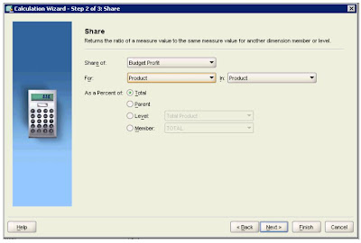
The Share template prompts you for the components you need to specify the calculation:
Share Of: A measure or calculated measure that is dimensioned by the Product dimension (in this example)

• For: The dimension for which the share is to be calculated
• In: The hierarchy to be used while calculating the share for the selected dimension
• As a Percent of: The dimension member to be used as a baseline to calculate the share. Select one of the following choices:
• Total: Specifies that the baseline consists of the total of all items on the level that is associated with the current member (that is, the item for which the share is being calculated). This option is disabled for a dimension that has no hierarchies.
• Parent: Specifies that the baseline consists of the total on the level of the parent for the current member (that is, the item for which the share is being calculated). This option is disabled for a dimension that has no hierarchies.
• Level: Specifies that the baseline consists of the total of a level to be specified. Choosing this item requires the selection of a value in the associated drop-down list. This list displays the names of levels from the selected hierarchy for the selected dimension that are available for calculating the share. This option is disabled for a dimension that has no hierarchies.
• Member: Specifies that the baseline consists of the total for a dimension member to be specified. Choosing this item requires the selection of a value in the associated drop-down list. This list displays the names of the dimension members that are available for calculating the share. This type of calculation applies to measures only.

Note that although the most common use of this template is to express the share as a “% of Total” or as a “% of Parent” in the chosen hierarchy, a specific member can be used as the baseline of the calculation. This is useful if you want to compare members of the dimension in question to a specific benchmark or model member, such as an established market leading product, flagship store, or key competitor.

So, as can be seen with this share calculation template it may be necessary to create multiple calculated measures using the same template to provide different results, such as shown below:


This report is showing the Budget Profit base measure and three Share calculations: Share of Product Total, Share of Product Level, and Share of a Product Member (Hardware). Note how the “% of Total,” “% of Level,” and “% of HW ” (hardware) category measures behave differently as the user drills down the product hierarchy. Also note that the third share measure on the report is base-lined to a specific product: the Hardware category. The report shows how Hardware compares to the other categories: Electronics, Peripherals and Accessories, Photo, and Software/Other.

Creating a % Different Prior Period Calculation
Using the “Percent Difference from Prior Period” calculated measure template, you can create a calculated measure that is useful to indicate growth or decline of a business over time. This calculation template is found in the Prior/Future Time Period calculation type folder. This template accepts input for the following items to calculate the percentage difference from a prior period:

• Measure: Select a measure or a dimension member for which you want to calculate the percentage difference from the prior period.
• Over: If there is more than one time dimension, then a box appears to enable the selection of the proper Time dimension. Otherwise, the default Time dimension is used.
• In: Select the hierarchy for the specified dimension.
• From: Choose one of the following items to indicate the previous time period that the comparison is to be based on:
• Year ago: Use if your measure is to compare performance with the same time period from the previous year
• Period ago: Use if your measure is to compare performance with the previous period at the same level in the Time hierarchy
• Number of periods or years ago: Use if your measure is to calculate a comparison with a time period of a specified number (entered in the number box) of periods ago, at a particular level (such as Year, Quarter, or Month)

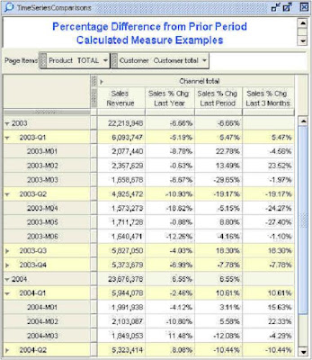
In a report this would look like this:



This report contains calculations of a number of alternative percentage differences from prior periods. All the measures automatically handle the situation in which the user needs to drill down into the time dimension and look at time periods at different levels. A single calculated measure in the AW can be used at any level of time, by any query tool, including SQL tools.

Note the following:

• The Last Year calculation works at all levels of time, and compares each time period with the same time period 1 year ago.
• The Last Period calculation works at all levels of time, and compares each time period with the previous period at the same level.
• The 3 Months Ago calculation works at the appropriate levels of time (in this case, Month and Quarter because a quarter is made up of three months), and compares each time period with the same time period 3 months ago (which is equivalent to one quarter ago).
• Similar calculations can be easily generated for Costs, Quantity, Profit, and Budget measures.

Creating a Moving Average Calculation
The Moving Average calculated measure template enables you to create moving averages over any of the measures in your AW. Moving averages are very useful when you analyze volatile data, because they smooth out the peaks and troughs and enable you to more easily visualize the trend in data. In the Moving Average template, you are asked to provide the following input:

• Measure: Select the measure for which you want to calculate a moving average.
• Over Time In: If there is more than one time dimension, then a box appears to enable the selection of the proper time dimension. Otherwise, the default time dimension is used. In identifies the hierarchy for the specified dimension.
• Include Previous: Enter the number of periods to be used for the calculation.
• An example of this calculation is as follows:
• Moving average of sales for the last three months = (Jan sales + Feb sales + March sales) / 3

Note: Similar pages are used for Moving Totals, Moving Maximums, and Moving Minimums.



Below is a combination graph showing how moving averages can be a useful way of smoothing out volatile data, thus enabling you to see the trends in data more easily.
One line is a moving six-month average, and the other line is a three-month average.




Modifying a Calculated Measure
Existing calculated measures can be edited from within AWM 10g. The descriptions and the calculation details can be changed. To change a calculated measure, click the calculated measure in the Model view. You see the general information displayed on the right. You can:

1. Make changes to labels and description. You can change the labels and description, but not the name.
2. Click the Launch Calculation Editor button to change the details of the calculated measure. You can change the details, but not the type, of the measure.

Managing Calculated Measures
My recommendation is always to create your calculated measures in a separate cube. This helps insulate you from changes to the physical implementation of your base cubes. For example, if you want to change the storage definition for a cube AWM forces you to delete the cube, which if it contains calculated measures means these are also delete and need to be recreated. By keeping your calculated measures in a separate cube it is possible to delete and a rebuild a cube without impacting the calculated measures. Assuming of course you do not change the dimensionality.

There are other ways to resolve this issue (deleting a cube but keeping the calculated measures):

• Save the calculated measure to an XML template
• Hack the XML definition for the cube

Saving the calculated measures to an XML file is always a good idea since this creates a backup of the definition. However, you can only save one measure at a time which is fine if you create the XML template when you define the calculated measure but not so good if you have lots and lots of calculated measures in a cube and then you decide to save them all to XML templates.

Hacking the XML is not something I would normally recommend, however, it is possible to move calculated measures from one template file to another using notepad. Again, assuming you do not change the dimensionality (as some measures may refer to specific dimensions and/or levels and/or hierarchies) you can cut & paste the XML. The calculated measures are all defined in the last but one block of the XML definition, using the tag “DerivedMeasure”. Simply copy all the DerivedMeasure blocks to your new cube XML template and reload that template to restore all your calculated measures. This works for 10gR2 but has not been tested with 11g.


Creating custom calculated Measures
Oracle OLAP Option has a very powerful calculation engine that supports a huge library of functions:

• Numeric Functions
• Time Series Functions
• Text Functions
• Financial Functions
• Statistical Functions
• Date and Time Functions
• Aggregation Functions
• Data Type Conversion Functions

Any these functions can be used to create a custom calculated measure. To get more information on these various functions you can refer to the Oracle OLAP DML Reference 10g Release 2 documentation:

http://download.oracle.com/docs/cd/B19306_01/olap.102/b14346/toc.htm

and for 11g:

http://download.oracle.com/docs/cd/B28359_01/olap.111/b28126/toc.htm

Here is a very simple example of how to create a custom calculated measure. Lets create a measure to show the percent variance for a measure, sales revenue, based on the prior-period. To do this we need to use the lagpct function. The LAGPCT function returns the percentage difference between the value of a dimensioned variable or expression at a specified offset of a dimension prior to the current value of that dimension and the current value of the dimensioned variable or expression.

The syntax for the function is :

• LAGPCT(variable, n, [dimension], [STATUS|NOSTATUS|limit-clause] )

Where

• Variable - A variable or expression that is dimensioned by dimension.
• ‘n’ - The offset (that is, the number of dimension values) to lag. LAGPCT uses this value to determine the number of values that LAGPCT should go back in dimension to retrieve the value of variable. Typically, n is a positive INTEGER that indicates the number of time periods (or dimension values) before the current one. When you specify a negative value for n, it indicates the number of time periods after the current one. In this case, LAGPCT compares the current value of the time series with a subsequent value.
• Dimension - The dimension along which the lag occurs. While this can be any dimension, it is typically a hierarchical time dimension of type TEXT that is limited to a single level (for example, the month or year level) or a dimension with a type of DAY, WEEK, MONTH, QUARTER or YEAR. When variable has a dimension with a type of DAY, WEEK, MONTH, QUARTER, or YEAR and you want LAGPCT to use that dimension, you can omit the dimension argument.
• Status can be one of the following:
• STATUS - Specifies that LAGPCT should use the current status list (that is, only the dimension values currently in status in their current status order) when computing the lag.
• NOSTATUS - (Default) Specifies that LAGPCT should use the default status (that is, a list all the dimension values in their original order) when computing the lag.
• limit-clause - Specifies that LAGPCT should use the default status limited by limit-clause when computing the lag. You can use any valid LIMIT clause (see the entry for the LIMIT command for further information). To specify that LAGPCT should use the current status limited by limit-clause when computing the lag, specify a LIMIT function for limit-clause.

Based on this syntax, the format of our function would be as follows:

• lagpct(sales_revenue, 1, TIME, LEVELREL TIME_LEVELREL)

since sales_revenue is the variable, we need to offset by one period to get the prior period, the dimension for the lag is Time and the limit clause is based on the standard form level object TIME_LEVELREL which ensures the correct prior period is selected based on the level of the dimension member, so months are only compared to months and quarters only compared to quarters and so on.

How do you install a Custom Calculation?
There are two ways to add a custom calculation to a cube:

• Special XML Template
• Excel Utility

It is possible to use an XML template file to define a custom calculated measure. As we noted in the XML definition of a cube containing a calculated measure the tag “DerivedMeasure” is used to denote a calculated measure. The template needs to have the following fields:

• Name
• LongName
• ShortName
• PluralName
• Id
• DataType
• IsInternal
• UseGlobalIndex
• ForceCalc
• ForceOrder
• SparseType
• AutoSolve
• IsValid
• ExpressionText

So for our example the following entries would be required:

• Name="SR_PPV_PCT"
• LongName="Sales Revenue Prior Period % Variance"
• ShortName=" Sales Rev Prior Period % Var"
• PluralName=" Sales Revenue Prior Period % Variance"
• Id="SALES.SR_PPV_PCT.MEASURE"
• DataType="Decimal"
• isInternal="false"
• UseGlobalIndex="false"
• ForceCalc="false"
• ForceOrder="false"
• SparseType="STANDARD"
• AutoSolve="DEFAULT"
• IsValid="true"
• ExpressionText=" lagpct(sales_revenue, 1, TIME, LEVELREL TIME_LEVELREL)"/>

Note the following:

• Name is can must match the “custom_calculated_measure_name” value in the Id tag.
• Id is derived as follows:
• Cube_name.custom_calculated_measure_name.MEASURE
• ExpressionText can refer either to the AWM Object View names or the physical objects from the ModelView. It can be more efficient to refer directly to the stored variables rather than using the standard form objects since this involves and additional layer of processing that is not always necessary. But start by referring to the standard form objects and check query performance before pointing directly to the base storage objects.

Fortunately, there is a much easier way to install a custom calculated measure. On OTN there is an Excel utility to that can help. See the link on the OLAP OTN Home Page, “Creating OLAP Calculations using Excel”:

http://download.oracle.com/otn/java/olap/SpreadsheetCalcs_10203.zip

Follow the instructions in the readme file and then open the spreadsheet included in the zip. This utility can be used to install both custom and standard calculations (those generated by the Calculated Measure Wizard), which makes installing calculations into a cube a quick and simple exercise. However, you do need to understand how the underlying functions are implemented as some of the templates require you to provide inputs such as “offset”, “start”, “stop” and “step”. Now the example worksheet provided does include examples for each of the types of templates, which makes it much easier to understand the values required for some of these templates. Using Excel is a good way to back up all your calculation definitions and makes it very easy to install the calculations into different environments, such as test, training,QA, production etc.

To use this utility follow these steps:

Step 1: Define your connection



This should match the details you set in AWM to connect to your analytic workspace.

Step 2: Select an AW


Once the connection is established the next stage is to select an AW. Each user is not limited to owning and/or using just one AW. In most implementations an OLAP user may have access to multiple AWs. Therefore, it is important to select the required AW before creating any calculations. A pulldown list of available AWs is provided just below the “Connection Details” button.

Step 3: Defining the calculation type
This utility will allow you to create both custom and pre-defined calculations. The column headed “Calculation Type” can be toggled between two values:

• Template
• Equation

The “Template” option will install one of the calculations from the AWM Calc Wizard and the “Equation” option allows you to define a free format equation.

Step 4: Basic details.
Each measure needs to have a name (which is the physical storage name for the measure so it cannot contain spaces or certain characters such as %, $, £ etc.), long label a short label and be assigned to a specific cube.



A pulldown list can be used to select the target cube. The next column to the right allows you to assign the measure to a measure folder.

Step 4a: Template Calculations
If you are defining a calculation based on a template, a pulldown list of available templates is available in the column marked “Calculation Template”



At this point it is a good idea to refer to the sample worksheet as this show you how to complete the additional columns to the right that manage the arguments for the templates:


The inputs are:

• Base measure – a pulldown list of all available measures is provided
• Dimension – the base dimension, which for most of the templates tends to be Time (pulldown list is available)
• Hierarchy – the main hierarchy from the time dimension (pulldown list is available)
• Level – the target level from the time dimension (pulldown list is available)
• Other numeric arguments determined by the type of template

All this information is taken from the Calculation Wizard so if you want to check your inputs simply run the calculation wizard in AWM and note the inputs for the specific template.

Step 4b: Equation Templates:
To create a custom calculation set the calculation type to “Equation” and then in the “Free Form Equation” column enter the formula using either the standard form object names or the physical storage object names. The equations can be one of three basic data types:

• Decimal
• Integer
• Text

In the example below (taken from the sample spreadsheet) two calculated measures are defined, one decimal and one text:



Measure name = PROFIT
Equation = SALES.SALES.MEASURE - SALES.COST.MEASURE
Data Type = DECIMAL

Measure Name = HOW_IS_MARGIN
Equation = If SALES.PROFIT.MEASURE/SALES.SALES.MEASURE gt .2 then 'GROOVY' else if SALES.PROFIT.MEASURE/SALES.SALES.MEASURE lt .1 then 'YIPES' else 'WHATEVER'
Data Type = TEXT

Step 5: Installing the Calculated Measures
Once all your calculations are defined, simply on the “Define Calculations” button.



This will launch a command window where the OLAP AW XML Java API is used to load the calculated measures defined in the worksheet into the target AW. During the installation process, feedback is written to the command window. An errors will be visible in this window and need to be resolved before trying the installation process again. This utility will overwrite an existing calculated measure so updating an AW is quick and easy since there is no need to first delete any existing calculated measures.

Once the measures have been deployed I would recommend starting AWM and checking all the calculated measures were correctly installed and do in fact return data. Sometimes it is easier to do this via the OLAP Worksheet, especially checking the data, since you can limit the various dimensions to a nice small subset of the data.

It is possible for a calculated measure to be installed and visible in AWM but not physically present. Which seems a little odd. This usually implies an issue with the naming convention, which allowed the object to be added to the metadata catalog, but the physical name generated an error for some reason. Easiest solution is to delete the calculated measure using AWM and try again after checking the name in the Excel worksheet.