More on the Calculated Measure Cube

In Keith's post, he describes how to create a calculated measure cube in Oracle 10g. In this post, I will describe how to create a calculated measure cube in Oracle 11g.

The basic technique is the same as Keith describes:

• Create a dimension representing calculations.
  Create a cube that will contain the stored measures.
• Create a reporting cube that will contain the calculated measures.
• Define the calculations.

Where the 11g technique varies from the 10g technique is how the calculations are defined. In 10g, the calculations are defined in OLAP DML code. In 11g, they are defined using the new calculation expression language. No OLAP DML programming is required. Also, in 11g, the SQL view is created and managed by the database so I get to skip the step of creating the view.

In this example, I have a cube that is dimensioned by time, product, customer and channel and base measures sales, units and costs. I want to add time series calculations to these base measures.

Step 1 - Creating the calculation dimension

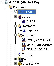
In my example, I have a calculation dimension. It plays the same role as Keith's Time View dimension - it's members represent calculations. The dimension is very simple, with one level and one hierarchy (which I really don't even need) and an attribute used for sorting.



The data for the calculation dimension looks like this:

Step 2 - Create cube for the stored measure

In this example, I have a UNITS_CUBE cube dimensioned by time, product, customer and channel with the stored measures sales, units and costs. This is mapped to a table that contains these measures and data is loaded into this cube.

Step 3 - Create the cube for the calculations

This second cube is dimensioned by time, product, customer, channel and calculation and calculated measures. This will be the cube used for reporting purposes. Oracle 11g automatically creates a SQL view of this cube.

Since this cube contains only stored measures settings such as partitioning, compression, sparsity and aggregation are irrelevant. The cube is not mapped to source tables.

In this cube, I created one calculated measure for each stored measure in the UNITS_CUBE. I named these SALES_CALCS, UNITS_CALCS and COST_CALCS. Note the two cubes below.



Here is where 11g is a lot different from 10g. The calculation definition of the calculated measures is defined in AWM as 11g OLAP calculation expressions. The expression uses the CASE statement to choose the calculation expression based on the value of the calculation dimension.

CASE

WHEN CALCULATION.DIM_KEY = 'BASE'
THEN UNITS_CUBE.SALES

WHEN CALCULATION.DIM_KEY = 'PP'
THEN LAG(UNITS_CUBE.SALES, 1) OVER HIERARCHY ("TIME".CALENDAR)

WHEN CALCULATION.DIM_KEY = 'CHG_PP'
THEN LAG_VARIANCE(UNITS_CUBE.SALES, 1) OVER HIERARCHY ("TIME".CALENDAR)

WHEN CALCULATION.DIM_KEY = 'PCT_CHG_PP'
THEN LAG_VARIANCE_PERCENT(UNITS_CUBE.SALES, 1) OVER HIERARCHY ("TIME".CALENDAR) * 100

ELSE NULL
END

Notes:

• The calculation expressions are based on the logical model, so you have none of the concerns that come with writing to the physical model of the AW (e.g., migration problems that occur when the physical model changes).
• The CASE statement is used to switch between calculations. CASE in the OLAP expression language is exactly the same as in SQL.
• Because the calculation is captured as on OLAP expression, it will be included in the XML template of the cube or AW.

The illustration below shows the calculation in the context of AWM and the cube.



In AWM, you can view the results. It looks like Keith's example, except that I've nested calculation under measure and put time down as rows. This shows some of the flexibility of this approach to modeling measures and calculations.



Updating INIT.ORA

Before querying your caclulated measure cube, add the following line to our init.ora file:

event="37395 trace name context forever, level 1024"

This line will control some looping code in the OLAP_TABLE table function that is used to query the cube using SQL. Without this line, null data can be returned by SQL for measures in the calculated meaure cube.

Displaying Data

This approach makes is very easy to define large numbers of calculations without cluttering the measure dimension. From a data display point of view, this approach really shines with a dimensionally aware tool such as the data viewer in AWM.

As the OLAP Option moves forward in time we find that almost all data is viewed in SQL based business intelligence tools such as Oracle Business Intelligence Enterprise Edition (OBI EE). What does this mean for data display?

If we think about OBI EE as an example of relational reporting tools that are commonly used with OLAP cubes, you have two choices: relational style reporting and pivot table style reporting.

With relational style reporting, the measures of this cube will appear as columns and the calculations as rows (because calculation is a dimension). This enables reporting in the context of a table. Note the calculation column.

The OBI EE pivot table offers additional flexibility. Note that this is the same report as in the AWM data viewer (above).



Which style reporting you use is, of course, up to you. With this cube, you can do either.

It is important to understand that tools such as OBI EE understand the fact columns from the cube view as measures and that they have no special understanding of the calculations dimension. Therefore, they don't typically offer measure formatting based on this column. In my example, I've sorted rows of the calculation dimension using the DISPLAY_ORDER attribute in the AW dimension (via the dimension view) and multiplied the percent change measure * 100 for display purposes.

Keep these types of issues in mind and you can add a lot of analytic capability to your SQL based BI applications and really take advantage of features such as the pivot table in OBI EE.