Friday, January 25, 2008
Oracle OLAP option - Did You Know?
Jameson White added "Did You Know?" to the DBA Zone on the Oracle OLAP option Wiki. Please make your comments in a thread on this Wiki page.
Thursday, January 24, 2008
OLAP Workshop 6 : Advanced Cube Design
In the previous workshop we looked at creating a cube making use of AWM’s ability to manage the other features. In most cases these default settings will provide good load and query performance. Certainly when looking at the data model that supports the 10g common schema the default settings do a great job and make life much easier. Consequently, you can design and build the analytic workspace from using the data sourced from the SH schema in about 15 minutes.
In some cases you may need to move beyond the default settings and in the next few sections we will look at the other tabs that are part of the Cube wizard. These tabs control sparsity, compression and partitioning features, aggregation rules, and summarization strategies. The tabs and the features they control will be explained in the following order:

But before proceeding there is one important thing you should always do before starting to load data into a cube (of a dimension) – review the data in as much detail as possible. Data quality is a subject that most companies often don’t even consider when building cubes, and most consultants just take the data given to them a load it without question.
In any project I would allocate 10-30% of the time looking at the data. The information gained at this stage will provide huge benefits later when you need to determine sparsity patterns (explained later). On a recent customer project I was asked to tune a cube to improve load and aggregation times. When we started to review the data we noticed some very very large numbers in one of the measures, which were simply amazing. After a lot of analysis we determine the ETL that was computing the figure in to the fact table had a mistake. Unfortunately both the developers and business users failed to identify this error. To compound the problem, the data formed a key business metric.
Therefore, NEVER EVER start loading data until you have checked the quality. Ideally you should use the data quality features of Warehouse Builder, which can significantly speed up this process. There are a number of presentations relating to data quality on the Warehouse Builder OTN home page.
Implementation Details Tab
Most of the advanced options for tuning your multidimensional model are found on the Implementation Details tabbed page of the Create Cube wizard. As shown below the Implementation Details tabbed page contains four important tuning features of Oracle OLAP. The correct use of these features ensures that your analytic workspace is very efficient and is implemented in an optimal way.

1.Sparsity: AWM 10g, by default, applies the common best practice in deciding which of your dimensions should be marked as “sparse” when you create a cube. Sparsity refers to the natural phenomenon evident in all multidimensional data to some degree: Not all the cells in the logical cube (the total possible combinations of all the dimension members for each dimension of the cube) will ever contain data. It is very common for a relatively small percentage of the possible combinations to actually store data. By understanding the sparsity of the data you expect to load into your AW, you can tune how it handles that sparsity and improve the performance of data loading and aggregation and reduce the disk-storage requirements for the populated AW.

After you understand which dimensions are sparse and which are not, their order can be important. When there are a large number of empty cells in a cube, the cube is said to be “sparse.” For example, if you are a manufacturer of consumer-packaged goods, you do not sell one or more of every single product you make to every customer, every day, through every sales channel. Different customers buy different products, at different time intervals, and each customer probably has a preferred channel. Different products may display different sparsity patterns: Ice creams and cold drinks tend to sell faster in the summer, whereas warm arctic coats are more popular in the winter (particularly in cold locations).
When using multidimensional technology, pay attention to sparsity so that you can design cubes efficiently. The effect of sparsity in data (and a badly designed cube) can result in tremendous growth in disk usage and a corresponding increase in the time taken to update and recalculate data in the cube. Inefficient sparsity control in any multidimensional data store can result in many empty cells actually being physically stored on the disk. This is something that is less of a concern with relational technology, because it is rare to store a completely null row in a table.
Oracle OLAP automatically deals with sparsity up to a point. But you, as a cube builder, can provide Oracle OLAP with the information that you know about your data (and information that Oracle OLAP needs to know) to deal with that data extremely efficiently.
Cube designers express sparsity in percentage terms. Data is said to be 5% dense (or 95% sparse) if only 5% of the possible combinations of the cells in a multidimensional measure or cube actually contain data. In many cases, data is very sparse, especially sales and marketing data. Only very aggregated data with a fairly small number of dimensions is typically dense enough for you to not consider sparsity.
Sparsity tends to increase with the number of dimensions and with the number of levels and hierarchies in each dimension. As you add dimensions to the definition of a cube, the number of possible cell combinations can increase exponentially. Also, the granularity of data affects sparsity. Low-level, detailed data is much more sparse than aggregate data. Very aggregate data is typically dense. Particular combinations of dimensions typically have different sparsity from others. For example, Time dimensions and Line dimensions are often more dense than dimensions such as Product, Customer, and Channel. This is because combinations of customers and products are sparser than combinations of customers and time or sparser than combinations of products and time. For this reason, AWM 10g asks you to confirm which of the dimensions for your data are sparse dimensions and which ones are dense.
In most cases I would recommend making all dimensions sparse. However, there are some additional considerations. The most important is the use of partitioning and we will look at this in one of the following sections. Sometimes, you may need to build a cube with different sparsity settings to determine the most efficient settings. In some cases making Time dense will generate a highly efficient cube and in other situations it will cause the massively extend the time take to load and aggregate data. The best method is to use an iterative development approach, but as with tuning be careful not to change too many settings at once as it becomes difficult to interpret the results.
A very common mistake I see with many customers is they insist on loading a zero balance into a measure. This is quite pointless, since a zero balance does not impact the overall total. Now it can be important to differentiate between an NA row and zero-row but for 99.9% of analysis it is possible to infer one from the other. Therefore, when loading data into a cube add an additional filter to remove zero and NA rows since this will provide huge savings in load and aggregation times. I was working on a project recently where a fact table contained 75 million rows of data and 65% of those rows contained 0 or NA.
2.Dimension order: It is possible to improve the build and aggregation performance of your AW by tuning the order in which the dimensions are specified in your cube.

When using the compression feature (discussed below), it is usually best to have a relatively small, dense dimension (such as Time) first in the list, followed by a group of all the sparse dimensions. Furthermore, it is generally the best practice to list the sparse dimensions in order of their size: from the one with the least members to the one with the most..
Note 1: Sparsity and dimension order are generally considered at the same time, which is why these choices are grouped together in the AWM 10g user interface:
My recommendation is to try building your cube with Time marked sparse and then try with Time marked dense. The effect on load times varies according to nature of the source data. I recently worked on a project where we marked all the dimensions as sparse and loaded a trial data set in 4 hours. By making Time dense, the same dataset loaded in 1 hour. Therefore, it pays to understand your data. But, most importantly, don’t assume you will get the data model right first time.
3.Compressed cubes and Global Composites: Version 10g of Oracle OLAP provides a new, internationally patented technology for the AW, which is exposed via a simple check box in AWM.

This is an extremely powerful data storage and aggregation algorithm optimized for sparse data. It is a new technology that is often dramatically faster than any previous OLAP server technology when aggregating sparse multidimensional data. The use of this feature can improve aggregation performance by a factor of 5 to 50. At the same time, query performance can improve, and disk storage is often also dramatically reduced. This feature is ideal for large volumes of sparse data but not suitable for all cubes (especially dense cubes).
If the “Use Compression” option is selected, then additional efficiency can often (but not always) be achieved by marking all dimensions (including Time) as sparse, especially for sparse data where there is known seasonality in the data, and especially if your AW is also partitioned on Time. But see my previous notes regarding this subject.
As we use this feature on more and more projects it is becoming clear that just about every cube will benefit from compression. Now there are some exceptions, such as cubes where you plan to use and application to write-back data directly into the cube, but such situations are easily managed by posting the updated data to a relational table and using the normal data load procedures to import and aggregate the data.
Note: Dimension order is unimportant when using compression. The multidimensional engine automatically determines how best to physically order the data after it is loaded.

A composite is an analytic workspace object used to manage sparsity. It maintains a list of all the sparse dimension-value combinations for, which there is data. By ignoring the sparse “empty” combinations in the underlying physical storage, the composite reduces the disk space required for sparse data. When data is added to a measure dimensioned by a composite, the AW automatically maintains the composite with any new values.
A “global” composite is simply a single composite for all data in a cube. Depending on the Compression and Partitioning choices you make, the behaviour of AWM will vary.
When would you opt to create Global Composites? The answer is very rarely. It can be beneficial to select this option in the case of a non-compressed cube that is partitioned. But as stated above, it is probably best to use compression on just about every cube you create, so you should probably leave the option unselected.
4.Partitioned cubes: You can partition your cube along any level in any hierarchy for a dimension. This is another way of improving the build and aggregation performance of your AW, especially if your computer has multiple CPUs. Oracle Database 10g (and thus the OLAP option) can run on single-CPU computers, large multi-CPU computers, and (with Real Application Clusters and Grid technology) clusters of computers that can be harnessed together and used as if they are one large computer. Oracle OLAP is, therefore, perhaps the most scalable OLAP server available.

Using partitioning does have certain knock-on consequences in 10g, but these are resolved in11g. In 10g, when you look at the “Summarize To” tab (this will be explained later) the levels above the partition key cannot be pre-aggregated and have to be solved at query time. Therefore, it is critical to select an appropriate level as the partition key so that query performance is maintained. Let us consider the example of time dimension:

If we use Day as the partition key, each individual partition will be small which should improve load times and aggregation times. But when a user creates a query based on yearly data 365 values have to be aggregated at run time for each cell being referenced within the query. Depending on the hardware this might or might not provide acceptable query performance.
If we use month as the partition key, each individual partition will still be relatively small and load times and aggregation times should still be acceptable. Each partition will hold between 28-31 days worth of data and in this case it would be prudent to make Time sparse within the model. However, when a user creates a query based on yearly data only 12 values have to be aggregated at run time for each cell being referenced within the query.
Partitioning has a big impact on two key areas:
Parallel Processing – By partitioning a cube, it is possible to solve it in parallel assuming data is being loaded into more than one partition. Which brings us to an important point. Most customers will typically partition their cubes by time. Of course if you only load data for one month at a time and use month as the partition key then parallel processing is not going to occur. Which may or may not be a good thing.
Rules Tab
On the Rules tabbed page, you identify aggregation rules for the cube (this is also available within each individual measure). You have many different kinds of aggregations available. This is one of the most powerful features of Oracle OLAP, enabling different dimensions to be independently calculated using different aggregation methods (or not using aggregation at all). In effect, a different aggregation method can be applied each dimension within a cube. The engine itself is also capable of supporting dimension member level aggregation plans through the use of MODELS. However, at this point in time Analytic Workspace Manager 10g does not support this feature. But AWM11g will support the ability to create dimension member aggregation plans in the form of custom aggregates.
In this image below, the aggregation method of SUM is used across all dimensions.

However, as we will see later different aggregation methods are available. For example, if you have costs and price data, you may want to see this data averaged over time, answering such business questions as “What is the average cost over 12 months?” or “What is the average price over 2 years?”
Aggregation Methods
It is common to set the aggregation rules only once for all measures contained in a cube. When you define a cube, you identify an aggregation method and any measures that you create that belong to the cube automatically receive the aggregation methods for that cube. This is the default behaviour, and it is one of the benefits of using a cube: By setting up aggregation rules and sparsity handling for all the measures once at the “cube” level, you save time and reduce the scope for errors or inconsistencies.

The default for aggregation used by AWM is the SUM method (simple additive aggregation) for each dimension. However, you do not have to aggregate data. Some measures have no meaning at aggregate levels of certain dimensions. In such cases, you can specify that the data is non-additive and should not be aggregated over those dimensions at all. Choosing the non-additive aggregation method means that when you view the data in the analytic workspace, you find data only at the leaf levels of the dimensions for which you selected that method.
Understanding Aggregation
AWM allows you to set aggregation rules for each dimension independently for your cubes and measures. That is, each dimension, if required, can use a different mathematical method of generating data for the parent and ancestors.
Here are some examples of different aggregation methods:

Sales quantities and revenues are usually aggregated over all dimensions using the SUM method, whereas inventory or headcount measures commonly require a different method (such as LAST) on the Time dimension and SUM for the other dimensions. More advanced aggregation methods, such as weighted average, are useful when aggregating measures such as Prices (weighted by Sales revenue).
Different Aggregation for Individual Measures
However, you are not limited to specifying that all measures of a cube have the same aggregation method. When adding measures to the cube, you can specify a different aggregation method, and accept the defaults of all the other measure settings.
For example, it is not uncommon for a single cube to contain measures such as Sales Revenue, Sales Quantity, Order Quantity, and Stock/Inventory Quantity. All these measures will aggregate using the SUM method over all dimensions, except for the Stock/Inventory measure. This requires a LAST method on the Time dimension (and SUM on all the others). Using the Rules tab for the Stock measure you can override the default aggregation method for Time and set the method to LAST, while retaining all the all other default settings from the cube.
Note: The ability to override cube settings for individual measures is not supported in compressed-cubes. If you use compression, and one of your measures requires a different aggregation method, you need to create it in a separate cube.
Aggregation Operators
There are a number of different aggregation operators available to you for summarizing data in your AW. The following is a brief description of each of the operators.

Most dimensions within real world models will have multiple hierarchies. In the image below, there are two separate hierarchies on the Time dimension.
On the Aggregation Rules tabbed page, when creating a cube, you can specify which hierarchy or hierarchies should be used for aggregation for that cube’s measures. You should select one or more hierarchies for each dimension being aggregated. If you omit a hierarchy, then no aggregate values are stored in it; they are always calculated in response to a query.
Because this may reduce query performance, generally you should omit a hierarchy only if it is seldom used. The default behaviour of AWM 10g is to select all hierarchies.

Aggregating Measures with Data Coming in at Different Levels
There are other occasions where careful selection of the hierarchies to use in aggregation is important, especially for measure data that arrives into the AW at different levels of aggregation.
Suppose you have an AW that contains Budget and Actuals cubes for the purposes of variance analysis. The leaf level for Actuals is the Day level, but Budgets are set at the Monthly level. Initially, you created a single Time hierarchy in which Year is the highest level and Day is the lowest level:

This is perfect for the aggregation hierarchy for the Actuals measures. However, there is an issue with the Budgets measure. If data is loaded at the Month level, but this hierarchy is used for the aggregation of Budgets, then aggregation may begin at the Day level. All the empty cells for Budget at the Day level would be interpreted as zeros for the purposes of aggregating the data, resulting in new monthly totals being calculated as zero.
To handle this situation, a recommended approach is to create a second hierarchy that stops at the Month level specifically for the purposes of aggregating Budgets:

You must deselect the hierarchy containing the Day level on the Aggregation Rules tab for the cube or measure in question. Use the Day-level hierarchy for the Actuals measures only. The Day-level hierarchy is the primary or default hierarchy for end users because it enables drilling down to the Day level, and Budgets are available at Month, Quarter, and Year, exactly as required.
Summarize To Tab
Within all OLAP models you will need to balance the desire to aggregate absolutely everything and the time taken to load into a cube and then aggregate that data. In general, the less you choose to pre-summarize when loading data into the AW, the higher the load placed on run-time queries. In this scenario, queries are likely to be a bit slower and the load on the server at query time is likely to be greater (for example, each user query is likely to be asking the server to do more calculations at a given point in time). Pre-calculated summaries are instantly available for retrieval and are generally faster to query.
However, it does not necessarily follow that full aggregation across all levels of all dimensions yields the best query performance. In many cases, partial summarization strategies can provide optimal build and aggregation performance with little noticeable impact on query performance.

Many experienced OLAP cube builders make the following recommendations regarding summarization strategies:
When you build and test your AWs, it is a good idea to include time in your project plan to experiment with different summarization strategies. Estimating in advance the exact storage requirements and aggregation times of a multidimensional cube (especially a highly dimensional, sparse one) is extremely difficult. So, it is often the case that some tuning after data is properly understood improves the performance of builds and aggregations.
You can use a database package to help you plan your summarisation strategy. There are two procedures, part of the DBMS_AW package that can provide help and guidance:
Cache Tab
Caching improves run-time performance in sessions that repeatedly access the same data, which is typical in data analysis. Caching temporarily saves calculated values in a session so that you can access them repeatedly without recalculating them each time. You have two options:

In the next workshop we will review how to quickly and easily load data into a cube and then review some best practices for loading data within a production environment.
In some cases you may need to move beyond the default settings and in the next few sections we will look at the other tabs that are part of the Cube wizard. These tabs control sparsity, compression and partitioning features, aggregation rules, and summarization strategies. The tabs and the features they control will be explained in the following order:
- Implementation Details
- Rules
- Summarize To
- Cache

But before proceeding there is one important thing you should always do before starting to load data into a cube (of a dimension) – review the data in as much detail as possible. Data quality is a subject that most companies often don’t even consider when building cubes, and most consultants just take the data given to them a load it without question.
In any project I would allocate 10-30% of the time looking at the data. The information gained at this stage will provide huge benefits later when you need to determine sparsity patterns (explained later). On a recent customer project I was asked to tune a cube to improve load and aggregation times. When we started to review the data we noticed some very very large numbers in one of the measures, which were simply amazing. After a lot of analysis we determine the ETL that was computing the figure in to the fact table had a mistake. Unfortunately both the developers and business users failed to identify this error. To compound the problem, the data formed a key business metric.
Therefore, NEVER EVER start loading data until you have checked the quality. Ideally you should use the data quality features of Warehouse Builder, which can significantly speed up this process. There are a number of presentations relating to data quality on the Warehouse Builder OTN home page.
Implementation Details Tab
Most of the advanced options for tuning your multidimensional model are found on the Implementation Details tabbed page of the Create Cube wizard. As shown below the Implementation Details tabbed page contains four important tuning features of Oracle OLAP. The correct use of these features ensures that your analytic workspace is very efficient and is implemented in an optimal way.

1.Sparsity: AWM 10g, by default, applies the common best practice in deciding which of your dimensions should be marked as “sparse” when you create a cube. Sparsity refers to the natural phenomenon evident in all multidimensional data to some degree: Not all the cells in the logical cube (the total possible combinations of all the dimension members for each dimension of the cube) will ever contain data. It is very common for a relatively small percentage of the possible combinations to actually store data. By understanding the sparsity of the data you expect to load into your AW, you can tune how it handles that sparsity and improve the performance of data loading and aggregation and reduce the disk-storage requirements for the populated AW.

After you understand which dimensions are sparse and which are not, their order can be important. When there are a large number of empty cells in a cube, the cube is said to be “sparse.” For example, if you are a manufacturer of consumer-packaged goods, you do not sell one or more of every single product you make to every customer, every day, through every sales channel. Different customers buy different products, at different time intervals, and each customer probably has a preferred channel. Different products may display different sparsity patterns: Ice creams and cold drinks tend to sell faster in the summer, whereas warm arctic coats are more popular in the winter (particularly in cold locations).
When using multidimensional technology, pay attention to sparsity so that you can design cubes efficiently. The effect of sparsity in data (and a badly designed cube) can result in tremendous growth in disk usage and a corresponding increase in the time taken to update and recalculate data in the cube. Inefficient sparsity control in any multidimensional data store can result in many empty cells actually being physically stored on the disk. This is something that is less of a concern with relational technology, because it is rare to store a completely null row in a table.
Oracle OLAP automatically deals with sparsity up to a point. But you, as a cube builder, can provide Oracle OLAP with the information that you know about your data (and information that Oracle OLAP needs to know) to deal with that data extremely efficiently.
Cube designers express sparsity in percentage terms. Data is said to be 5% dense (or 95% sparse) if only 5% of the possible combinations of the cells in a multidimensional measure or cube actually contain data. In many cases, data is very sparse, especially sales and marketing data. Only very aggregated data with a fairly small number of dimensions is typically dense enough for you to not consider sparsity.
Sparsity tends to increase with the number of dimensions and with the number of levels and hierarchies in each dimension. As you add dimensions to the definition of a cube, the number of possible cell combinations can increase exponentially. Also, the granularity of data affects sparsity. Low-level, detailed data is much more sparse than aggregate data. Very aggregate data is typically dense. Particular combinations of dimensions typically have different sparsity from others. For example, Time dimensions and Line dimensions are often more dense than dimensions such as Product, Customer, and Channel. This is because combinations of customers and products are sparser than combinations of customers and time or sparser than combinations of products and time. For this reason, AWM 10g asks you to confirm which of the dimensions for your data are sparse dimensions and which ones are dense.
In most cases I would recommend making all dimensions sparse. However, there are some additional considerations. The most important is the use of partitioning and we will look at this in one of the following sections. Sometimes, you may need to build a cube with different sparsity settings to determine the most efficient settings. In some cases making Time dense will generate a highly efficient cube and in other situations it will cause the massively extend the time take to load and aggregate data. The best method is to use an iterative development approach, but as with tuning be careful not to change too many settings at once as it becomes difficult to interpret the results.
A very common mistake I see with many customers is they insist on loading a zero balance into a measure. This is quite pointless, since a zero balance does not impact the overall total. Now it can be important to differentiate between an NA row and zero-row but for 99.9% of analysis it is possible to infer one from the other. Therefore, when loading data into a cube add an additional filter to remove zero and NA rows since this will provide huge savings in load and aggregation times. I was working on a project recently where a fact table contained 75 million rows of data and 65% of those rows contained 0 or NA.
2.Dimension order: It is possible to improve the build and aggregation performance of your AW by tuning the order in which the dimensions are specified in your cube.

When using the compression feature (discussed below), it is usually best to have a relatively small, dense dimension (such as Time) first in the list, followed by a group of all the sparse dimensions. Furthermore, it is generally the best practice to list the sparse dimensions in order of their size: from the one with the least members to the one with the most..
Note 1: Sparsity and dimension order are generally considered at the same time, which is why these choices are grouped together in the AWM 10g user interface:
My recommendation is to try building your cube with Time marked sparse and then try with Time marked dense. The effect on load times varies according to nature of the source data. I recently worked on a project where we marked all the dimensions as sparse and loaded a trial data set in 4 hours. By making Time dense, the same dataset loaded in 1 hour. Therefore, it pays to understand your data. But, most importantly, don’t assume you will get the data model right first time.
3.Compressed cubes and Global Composites: Version 10g of Oracle OLAP provides a new, internationally patented technology for the AW, which is exposed via a simple check box in AWM.

This is an extremely powerful data storage and aggregation algorithm optimized for sparse data. It is a new technology that is often dramatically faster than any previous OLAP server technology when aggregating sparse multidimensional data. The use of this feature can improve aggregation performance by a factor of 5 to 50. At the same time, query performance can improve, and disk storage is often also dramatically reduced. This feature is ideal for large volumes of sparse data but not suitable for all cubes (especially dense cubes).
If the “Use Compression” option is selected, then additional efficiency can often (but not always) be achieved by marking all dimensions (including Time) as sparse, especially for sparse data where there is known seasonality in the data, and especially if your AW is also partitioned on Time. But see my previous notes regarding this subject.
As we use this feature on more and more projects it is becoming clear that just about every cube will benefit from compression. Now there are some exceptions, such as cubes where you plan to use and application to write-back data directly into the cube, but such situations are easily managed by posting the updated data to a relational table and using the normal data load procedures to import and aggregate the data.
Note: Dimension order is unimportant when using compression. The multidimensional engine automatically determines how best to physically order the data after it is loaded.

A composite is an analytic workspace object used to manage sparsity. It maintains a list of all the sparse dimension-value combinations for, which there is data. By ignoring the sparse “empty” combinations in the underlying physical storage, the composite reduces the disk space required for sparse data. When data is added to a measure dimensioned by a composite, the AW automatically maintains the composite with any new values.
A “global” composite is simply a single composite for all data in a cube. Depending on the Compression and Partitioning choices you make, the behaviour of AWM will vary.
When would you opt to create Global Composites? The answer is very rarely. It can be beneficial to select this option in the case of a non-compressed cube that is partitioned. But as stated above, it is probably best to use compression on just about every cube you create, so you should probably leave the option unselected.
4.Partitioned cubes: You can partition your cube along any level in any hierarchy for a dimension. This is another way of improving the build and aggregation performance of your AW, especially if your computer has multiple CPUs. Oracle Database 10g (and thus the OLAP option) can run on single-CPU computers, large multi-CPU computers, and (with Real Application Clusters and Grid technology) clusters of computers that can be harnessed together and used as if they are one large computer. Oracle OLAP is, therefore, perhaps the most scalable OLAP server available.

Using partitioning does have certain knock-on consequences in 10g, but these are resolved in11g. In 10g, when you look at the “Summarize To” tab (this will be explained later) the levels above the partition key cannot be pre-aggregated and have to be solved at query time. Therefore, it is critical to select an appropriate level as the partition key so that query performance is maintained. Let us consider the example of time dimension:

If we use Day as the partition key, each individual partition will be small which should improve load times and aggregation times. But when a user creates a query based on yearly data 365 values have to be aggregated at run time for each cell being referenced within the query. Depending on the hardware this might or might not provide acceptable query performance.
If we use month as the partition key, each individual partition will still be relatively small and load times and aggregation times should still be acceptable. Each partition will hold between 28-31 days worth of data and in this case it would be prudent to make Time sparse within the model. However, when a user creates a query based on yearly data only 12 values have to be aggregated at run time for each cell being referenced within the query.
Partitioning has a big impact on two key areas:
- Partial Aggregation
- Parallel Processing
Parallel Processing – By partitioning a cube, it is possible to solve it in parallel assuming data is being loaded into more than one partition. Which brings us to an important point. Most customers will typically partition their cubes by time. Of course if you only load data for one month at a time and use month as the partition key then parallel processing is not going to occur. Which may or may not be a good thing.
Rules Tab
On the Rules tabbed page, you identify aggregation rules for the cube (this is also available within each individual measure). You have many different kinds of aggregations available. This is one of the most powerful features of Oracle OLAP, enabling different dimensions to be independently calculated using different aggregation methods (or not using aggregation at all). In effect, a different aggregation method can be applied each dimension within a cube. The engine itself is also capable of supporting dimension member level aggregation plans through the use of MODELS. However, at this point in time Analytic Workspace Manager 10g does not support this feature. But AWM11g will support the ability to create dimension member aggregation plans in the form of custom aggregates.
In this image below, the aggregation method of SUM is used across all dimensions.

However, as we will see later different aggregation methods are available. For example, if you have costs and price data, you may want to see this data averaged over time, answering such business questions as “What is the average cost over 12 months?” or “What is the average price over 2 years?”
Aggregation Methods
It is common to set the aggregation rules only once for all measures contained in a cube. When you define a cube, you identify an aggregation method and any measures that you create that belong to the cube automatically receive the aggregation methods for that cube. This is the default behaviour, and it is one of the benefits of using a cube: By setting up aggregation rules and sparsity handling for all the measures once at the “cube” level, you save time and reduce the scope for errors or inconsistencies.

The default for aggregation used by AWM is the SUM method (simple additive aggregation) for each dimension. However, you do not have to aggregate data. Some measures have no meaning at aggregate levels of certain dimensions. In such cases, you can specify that the data is non-additive and should not be aggregated over those dimensions at all. Choosing the non-additive aggregation method means that when you view the data in the analytic workspace, you find data only at the leaf levels of the dimensions for which you selected that method.
Understanding Aggregation
AWM allows you to set aggregation rules for each dimension independently for your cubes and measures. That is, each dimension, if required, can use a different mathematical method of generating data for the parent and ancestors.
Here are some examples of different aggregation methods:
- SUM simply adds up the values of the measure for each child value to compute the value for the parent. This is the default (and most common) behaviour.
- AVERAGE calculates the average of the values of the measure for each child value to provide the value for the parent.
- LAST takes the last non-NA (Null) value of the child members and uses that as the value for the parent.

Sales quantities and revenues are usually aggregated over all dimensions using the SUM method, whereas inventory or headcount measures commonly require a different method (such as LAST) on the Time dimension and SUM for the other dimensions. More advanced aggregation methods, such as weighted average, are useful when aggregating measures such as Prices (weighted by Sales revenue).
Different Aggregation for Individual Measures
However, you are not limited to specifying that all measures of a cube have the same aggregation method. When adding measures to the cube, you can specify a different aggregation method, and accept the defaults of all the other measure settings.
For example, it is not uncommon for a single cube to contain measures such as Sales Revenue, Sales Quantity, Order Quantity, and Stock/Inventory Quantity. All these measures will aggregate using the SUM method over all dimensions, except for the Stock/Inventory measure. This requires a LAST method on the Time dimension (and SUM on all the others). Using the Rules tab for the Stock measure you can override the default aggregation method for Time and set the method to LAST, while retaining all the all other default settings from the cube.
Note: The ability to override cube settings for individual measures is not supported in compressed-cubes. If you use compression, and one of your measures requires a different aggregation method, you need to create it in a separate cube.
Aggregation Operators
There are a number of different aggregation operators available to you for summarizing data in your AW. The following is a brief description of each of the operators.

- Average: Adds data values, and then divides the sum by the number of data values that are added together
- Hierarchical Average: Adds data values, and then divides the sum by the number of children in the dimension hierarchy. Unlike Average, which counts only non-NA children, Hierarchical Average counts all the logical children of a parent, regardless of whether each child does or does not have a value.
- Hierarchical Weighted Average: Multiplies non-NA child data values by their corresponding weight values, and then divides the result by the sum of the weight values. Unlike Weighted Average, Hierarchical Weighted Average includes weight values in the denominator sum even when the corresponding child values are NA. You identify the weight object in the Based On field.
- Weighted Average: Multiplies each data value by a weight factor, adds the data values, and then divides that result by the sum of the weight factors. You identify the weight object in the Based On field.
- First Non-NA Data Value: The first real data value
- Hierarchical First Member: The first data value in the hierarchy, even when that value is NA
- Hierarchical Weighted First: The first data value in the hierarchy multiplied by its corresponding weight value, even when that value is NA. You identify the weight object in the Based On field.
- Weighted First: The first non-NA data value multiplied by its corresponding weight value. You identify the weight object in the Based On field.
- Last Non-NA Data Value: The last real data value
- Hierarchical Last Member: The last data value in the hierarchy, even when that value is NA
- Hierarchical Weighted Last: The last data value in the hierarchy multiplied by its corresponding weight value, even when that value is NA. You identify the weight object in the Based On field.
- Weighted Last: The last non-NA data value multiplied by its corresponding weight value. You identify the weight object in the Based On field.
- Maximum: The largest data value among the children of each parent
- Minimum: The smallest data value among the children of each parent
- Non-additive (Do Not Summarize): Do not aggregate any data for this dimension. Use this keyword only in an operator variable. It has no effect otherwise.
- Sum: Adds data values (default)
- Scaled Sum: Adds the value of a weight object to each data value, and then adds the data values. You identify the weight object in the Based On field.
- Weighted Sum: Multiplies each data value by a weight factor, and then adds the data values. You identify the weight object in the Based On field.
Most dimensions within real world models will have multiple hierarchies. In the image below, there are two separate hierarchies on the Time dimension.
On the Aggregation Rules tabbed page, when creating a cube, you can specify which hierarchy or hierarchies should be used for aggregation for that cube’s measures. You should select one or more hierarchies for each dimension being aggregated. If you omit a hierarchy, then no aggregate values are stored in it; they are always calculated in response to a query.
Because this may reduce query performance, generally you should omit a hierarchy only if it is seldom used. The default behaviour of AWM 10g is to select all hierarchies.

Aggregating Measures with Data Coming in at Different Levels
There are other occasions where careful selection of the hierarchies to use in aggregation is important, especially for measure data that arrives into the AW at different levels of aggregation.
Suppose you have an AW that contains Budget and Actuals cubes for the purposes of variance analysis. The leaf level for Actuals is the Day level, but Budgets are set at the Monthly level. Initially, you created a single Time hierarchy in which Year is the highest level and Day is the lowest level:

This is perfect for the aggregation hierarchy for the Actuals measures. However, there is an issue with the Budgets measure. If data is loaded at the Month level, but this hierarchy is used for the aggregation of Budgets, then aggregation may begin at the Day level. All the empty cells for Budget at the Day level would be interpreted as zeros for the purposes of aggregating the data, resulting in new monthly totals being calculated as zero.
To handle this situation, a recommended approach is to create a second hierarchy that stops at the Month level specifically for the purposes of aggregating Budgets:

You must deselect the hierarchy containing the Day level on the Aggregation Rules tab for the cube or measure in question. Use the Day-level hierarchy for the Actuals measures only. The Day-level hierarchy is the primary or default hierarchy for end users because it enables drilling down to the Day level, and Budgets are available at Month, Quarter, and Year, exactly as required.
Summarize To Tab
Within all OLAP models you will need to balance the desire to aggregate absolutely everything and the time taken to load into a cube and then aggregate that data. In general, the less you choose to pre-summarize when loading data into the AW, the higher the load placed on run-time queries. In this scenario, queries are likely to be a bit slower and the load on the server at query time is likely to be greater (for example, each user query is likely to be asking the server to do more calculations at a given point in time). Pre-calculated summaries are instantly available for retrieval and are generally faster to query.
However, it does not necessarily follow that full aggregation across all levels of all dimensions yields the best query performance. In many cases, partial summarization strategies can provide optimal build and aggregation performance with little noticeable impact on query performance.

Many experienced OLAP cube builders make the following recommendations regarding summarization strategies:
- Large dimensions, and those with many deep levels and/or hierarchies, are typically the most “expensive” to aggregate over. They are also likely to be one of the sparse dimensions in the cube definition. For such dimensions, a common guideline is to decide to summarize using a “skip-level” approach—that is, to precalculate every other level in the hierarchy. This generally gives reasonably good results and a solid basis for further tuning (if required)
- If there is a small, dense dimension (such as Time) as the first dimension on the list of dimensions for a cube, then it is often a good strategy to leave that dimension to completely summarize on the fly at run time, especially if a large number of sparse data-level combinations have been computed
When you build and test your AWs, it is a good idea to include time in your project plan to experiment with different summarization strategies. Estimating in advance the exact storage requirements and aggregation times of a multidimensional cube (especially a highly dimensional, sparse one) is extremely difficult. So, it is often the case that some tuning after data is properly understood improves the performance of builds and aggregations.
You can use a database package to help you plan your summarisation strategy. There are two procedures, part of the DBMS_AW package that can provide help and guidance:
- The SPARSITY_ADVICE_TABLE procedure creates a table for storing the advice generated by the ADVISE_SPARSITY procedure
- The ADVISE_SPARSITY procedure runs a series of queries against your data and make recommendations about what data to pre-summarize and what to leave for dynamic aggregation. The 11g release of Analytic Workspace Manager leverages this database feature and make recommendations directly inside the tool
Cache Tab
Caching improves run-time performance in sessions that repeatedly access the same data, which is typical in data analysis. Caching temporarily saves calculated values in a session so that you can access them repeatedly without recalculating them each time. You have two options:
- Cache run-time aggregations using session cache: This is the default behaviour. This option ensures that any run-time aggregations that are completed during a session are cached for the remainder of the session, improving query performance as the session progresses. This setting is ideal for a larger number of OLAP applications, namely those that allow read-only analysis where the underlying data is not changing during a session.
- Do not cache run-time aggregations: Select this option if the cube would be subject to what-if analysis and, therefore, it would be important that previously calculated summarizations are not reused.

In the next workshop we will review how to quickly and easily load data into a cube and then review some best practices for loading data within a production environment.
Monday, January 21, 2008
OLAP Workshop 5 : Building Cubes
In the last series of Workshops, we started to look at building the dimensions to support our data model. Each dimension contained levels and a hierarchy. The purpose of a hierarchy is to provide the relationships for summarization of measures in the cube and to make navigating multiple levels of data easy and intuitive for the end user. The next stage is to start building cubes.
Creating Cubes
What Are Cubes?
Cubes are containers of measures (facts). They simply provide a convenient way of collecting up measures with the same dimensions. Therefore, all measures in a cube are candidates for being processed together at all stages: data loading, aggregation, and storage. Cubes are only visible to the cube builder (end users only see the measures they contain) and simplify the setup and maintenance of measures in AWM.
Creating Cubes
To create a cube, right-click the Cubes node in the navigator, and then select the Create Cube option.

Note: You can also create a cube from a cube template if you have a template available.
The Create Cube window appears, as shown below:

The Create Cube wizard provides a tabbed page interface that enables you to specify the logical model and processing options for a cube. The best way to use this wizard is to always work from left to right across the various tabs.
General Tabbed Page
On the General tabbed page, enter the basic information about the cube:
The tick box “Use Default Aggregation Plan for Cube Aggregation” allows you to shortcut the process of creating of measures by applying the settings defined at the cube level to all measures within the cube. As we will see later, defining measures is an almost identical process as defining cube.
Translations Tabbed Page
Enables you to provide long and short descriptions for the cube in each language that the AW supports. Although there are other tabs within the cube wizard, at this point it is possible to ignore all the other tabs and allow the AWM to default all the other features.
Adding Measures to a Cube
Base measures store the facts collected about your business. Dimensions logically organize the edges of a measure, and the body of the measure contains data values. Each measure belongs to a particular cube, and by default all the settings for a measure (such as dimensions) are inherited from the cube.
Right clicking on the Measures node in the navigator can create a measure. Next select the Create Measure option.

This will then launch the wizard to create the measure:

General Tabbed Page
On the General tabbed page, you create a name and add label information. Long labels are used by most OLAP clients for display. If you do not specify a value for the long label, then it defaults to the measure’s name. Once the measure is defined you cannot change the name of the measure. If you delete a measure all the data associated with that measure is lost.
Other Tabbed Pages
The Translations tabbed page enables you to provide long and short descriptions for the measure in each language that the AW supports. The other tabbed pages (Implementation Details, Rules, and so on) enable the selection of certain measure-specific processing options other than the settings that are applied by the definition of the cube. These tabbed pages are examined in the following workshop.
At this point it possible to simply create the measure and allow AWM to default all the other settings.
Loading Data into a Cube.
After creating logical objects, you can map them to relational data sources in the Oracle database. Afterward, you can load data into your analytic workspace by using the Maintain Analytic Workspace Wizard.
Step 1 – Mapping Data Sources
To map your measures to a data source, perform these steps:
1. In the navigator, choose Mappings for the cube that contains the measure that you want to map. A list of schemas appears. Find the schema to which you want to map your measure, and then click the + button.
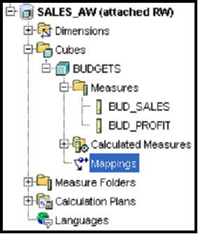
2. Select either Tables or Views, depending on what you are mapping to.

3. Find the table or view name and double-click, or drag it to the mapping canvas. When on the canvas, the structure of the table is visible.

Note: If you want to see the data in the table or view, right-click the name of the table or view, and then select the View Data option.
My recommendation is never to map directly to a fact table. Always use a view as this allows to you to fine tune the load process. For example by using a view you can select to load a single time period, which can be useful when you are trying to manage some of the more advanced settings and you are using an iterative development approach. As you will see later, using a view can make the data take stage (i.e. the initial build of the cube) easier to plan and manage.
4. Drag the cursor from the column name in the relational source to the destination object name in the measure. The image below shows a completed mapping.

Note: The mapping canvas enables you to map the contents of the source data to any level of dimensions. Here, because Budgets are set by product, and by channel for each month, map them to the Month, Product and Channel levels. In the next lesson there is advice techniques for managing situations where source data for different cubes and measures is loaded at different leaf levels of detail.
Step 2 - Loading Data into the Cube
AWM contains a data maintenance wizard to help you create a job to load data into your cubes. The job both loads and aggregates the data within the cube as a single job. You can load:

In this screenshot, the Budgets cube is maintained. This results in the loading of data for all the dimensions that organize the cube and all the mapped measures associated with the cube.

The Maintenance Wizard takes you through a set of steps to load data from the mapped relational objects to the multidimensional objects in the AW.
Step 1 of the wizard, you identify the objects for which data is to be loaded. If you choose cubes, all the measures for the cube are selected. Alternatively, you can choose a specific measure of a cube. After a measure or cube is selected, the associated dimensions are automatically selected as well. AWM, by default, selects the related dimensions for the cube. This is because AWM is dimensionally aware, and knows that the dimensions must exist and be populated in order for measures to be loaded (the dimensions organize the measures physically not just logically in an AW, so they must be maintained before the measure data can be loaded).
Note – My personal preference is not to maintain dimensions at the same time as processing the cube. This goes back to the old days of Express Server when it was best practice to load dimensions first and then load data as a separate job. The reason for this two-step process was to ensure efficient storage of a measure. With the OLAP Option I am not sure if this should still be considered best practice but old habits die-hard.
From this screen it possible to simply click on the “Finish” button and the job will run immediately. Alternatively you can step through the two other screens to set some additional processing options:

Step 2 allows you to determine how previously load data should be managed as well as new data. For the moment, simply ignore this screen, all will be explained in the next workshop.

Step 3 allows you to determine when to run the job. For the moment simply use the default option to run the job immediately. Again, the other options will be explained in the next workshop.

After the loading of data is completed, you can view the report which is shown below (this is the 10g report, the 11g report provides a lot more detail):

After successful completion, the data in your AW is ready to be analyzed.
Note - All the maintenance logging goes into the XML_LOAD_LOG table (for 10g, with 11g there have been some changes which will be explained in a later post), which belongs to the OLAPSYS user. This table can be reviewed later, if required. There is a lot of information in this log, but some of it can be hidden. Always make sure ALL your records were correctly loaded. The log file will tell you if any were rejected, but unfortunately it will not tell you why or which records. The usual reasons are:
Viewing the Results
After data is loaded, you can preview it by using the Data Viewer. To see the data, right-click the name of the measure or cube that you want to view, and then select View Data from the submenu.

A tabular report appears. If you view a cube, all measures in the cube are displayed. In the Data Viewer, you can:
Note - When you are developing an analytic workspace always check your data after it has loaded. Do not just assume the data is correct. It always good practice to go back to the fact table and make sure the totals from the source data match the totals in the OLAP cube.
In end-user tools and applications, more functionality (such as formatting, colour coding, and cell actions) is enabled in Discoverer Plus OLAP, as you see in the lesson titled “Building Analytical Reports with OracleBI Discoverer Plus OLAP.”

Note: From the File menu within the Data Viewer, or from the Query Builder tool,
you can access the Oracle OLAP Query Builder. This query wizard is used throughout Oracle Business Intelligence tools.

As shown in the image above, you drill down on data to the lowest levels of detail by clicking the arrow icon to the left of the dimension value. Notice that the measure appears to the user as fully aggregated at all level combinations of all dimensions. This is an important feature of the Oracle OLAP dimensional model. All data is presented to the end user as if it is already aggregated and calculated, even if some or all of the data being displayed is being calculated on the fly.
For example, some of the budget data has been pre-aggregated during the maintenance task, and some of it is being calculated dynamically. The end user cannot tell the difference, and does not need to know. The AW contains the data and the calculation logic and presents the results that the user needs. From the technical perspective, not even the query behind this crosstab needs to know whether the measure cells being requested are pre-computed or not. The query simply requests these cells from the database, and the AW engine performs any calculations required at query time.
In some cases you may need to move beyond the default settings described in this workshop. Therefore, in the next workshop we will look at the other tabs that are part of the Cube wizard. These tabs control sparsity, compression and partitioning features, aggregation rules, and summarization strategies.
Creating Cubes
What Are Cubes?
Cubes are containers of measures (facts). They simply provide a convenient way of collecting up measures with the same dimensions. Therefore, all measures in a cube are candidates for being processed together at all stages: data loading, aggregation, and storage. Cubes are only visible to the cube builder (end users only see the measures they contain) and simplify the setup and maintenance of measures in AWM.
Creating Cubes
To create a cube, right-click the Cubes node in the navigator, and then select the Create Cube option.

Note: You can also create a cube from a cube template if you have a template available.
The Create Cube window appears, as shown below:

The Create Cube wizard provides a tabbed page interface that enables you to specify the logical model and processing options for a cube. The best way to use this wizard is to always work from left to right across the various tabs.
General Tabbed Page
On the General tabbed page, enter the basic information about the cube:
- Provide the cube with a distinct name and provide the short and long label descriptions. Note – the name of the cube cannot be changed once the cube has been created.
- Identify the dimensionality of the cube by using the arrow keys to move dimensions from the Available Dimension list to the Selected Dimension list. After you define the dimensionality, all measures that you create based on this cube will have the same dimensionality. Note – the dimensionality of the cube cannot be changed once the cube has been created.
The tick box “Use Default Aggregation Plan for Cube Aggregation” allows you to shortcut the process of creating of measures by applying the settings defined at the cube level to all measures within the cube. As we will see later, defining measures is an almost identical process as defining cube.
Translations Tabbed Page
Enables you to provide long and short descriptions for the cube in each language that the AW supports. Although there are other tabs within the cube wizard, at this point it is possible to ignore all the other tabs and allow the AWM to default all the other features.
Adding Measures to a Cube
Base measures store the facts collected about your business. Dimensions logically organize the edges of a measure, and the body of the measure contains data values. Each measure belongs to a particular cube, and by default all the settings for a measure (such as dimensions) are inherited from the cube.
Right clicking on the Measures node in the navigator can create a measure. Next select the Create Measure option.

This will then launch the wizard to create the measure:

General Tabbed Page
On the General tabbed page, you create a name and add label information. Long labels are used by most OLAP clients for display. If you do not specify a value for the long label, then it defaults to the measure’s name. Once the measure is defined you cannot change the name of the measure. If you delete a measure all the data associated with that measure is lost.
Other Tabbed Pages
The Translations tabbed page enables you to provide long and short descriptions for the measure in each language that the AW supports. The other tabbed pages (Implementation Details, Rules, and so on) enable the selection of certain measure-specific processing options other than the settings that are applied by the definition of the cube. These tabbed pages are examined in the following workshop.
At this point it possible to simply create the measure and allow AWM to default all the other settings.
Loading Data into a Cube.
After creating logical objects, you can map them to relational data sources in the Oracle database. Afterward, you can load data into your analytic workspace by using the Maintain Analytic Workspace Wizard.
Step 1 – Mapping Data Sources
To map your measures to a data source, perform these steps:
1. In the navigator, choose Mappings for the cube that contains the measure that you want to map. A list of schemas appears. Find the schema to which you want to map your measure, and then click the + button.

2. Select either Tables or Views, depending on what you are mapping to.

3. Find the table or view name and double-click, or drag it to the mapping canvas. When on the canvas, the structure of the table is visible.

Note: If you want to see the data in the table or view, right-click the name of the table or view, and then select the View Data option.
My recommendation is never to map directly to a fact table. Always use a view as this allows to you to fine tune the load process. For example by using a view you can select to load a single time period, which can be useful when you are trying to manage some of the more advanced settings and you are using an iterative development approach. As you will see later, using a view can make the data take stage (i.e. the initial build of the cube) easier to plan and manage.
4. Drag the cursor from the column name in the relational source to the destination object name in the measure. The image below shows a completed mapping.

Note: The mapping canvas enables you to map the contents of the source data to any level of dimensions. Here, because Budgets are set by product, and by channel for each month, map them to the Month, Product and Channel levels. In the next lesson there is advice techniques for managing situations where source data for different cubes and measures is loaded at different leaf levels of detail.
Step 2 - Loading Data into the Cube
AWM contains a data maintenance wizard to help you create a job to load data into your cubes. The job both loads and aggregates the data within the cube as a single job. You can load:
- All mapped objects in the analytic workspace
- All mapped measures in a cube including the dimensions
- All mapped measures in a cube excluding the dimensions
- Individually mapped measures

In this screenshot, the Budgets cube is maintained. This results in the loading of data for all the dimensions that organize the cube and all the mapped measures associated with the cube.

The Maintenance Wizard takes you through a set of steps to load data from the mapped relational objects to the multidimensional objects in the AW.
Step 1 of the wizard, you identify the objects for which data is to be loaded. If you choose cubes, all the measures for the cube are selected. Alternatively, you can choose a specific measure of a cube. After a measure or cube is selected, the associated dimensions are automatically selected as well. AWM, by default, selects the related dimensions for the cube. This is because AWM is dimensionally aware, and knows that the dimensions must exist and be populated in order for measures to be loaded (the dimensions organize the measures physically not just logically in an AW, so they must be maintained before the measure data can be loaded).
Note – My personal preference is not to maintain dimensions at the same time as processing the cube. This goes back to the old days of Express Server when it was best practice to load dimensions first and then load data as a separate job. The reason for this two-step process was to ensure efficient storage of a measure. With the OLAP Option I am not sure if this should still be considered best practice but old habits die-hard.
From this screen it possible to simply click on the “Finish” button and the job will run immediately. Alternatively you can step through the two other screens to set some additional processing options:

Step 2 allows you to determine how previously load data should be managed as well as new data. For the moment, simply ignore this screen, all will be explained in the next workshop.

Step 3 allows you to determine when to run the job. For the moment simply use the default option to run the job immediately. Again, the other options will be explained in the next workshop.

After the loading of data is completed, you can view the report which is shown below (this is the 10g report, the 11g report provides a lot more detail):

After successful completion, the data in your AW is ready to be analyzed.
Note - All the maintenance logging goes into the XML_LOAD_LOG table (for 10g, with 11g there have been some changes which will be explained in a later post), which belongs to the OLAPSYS user. This table can be reviewed later, if required. There is a lot of information in this log, but some of it can be hidden. Always make sure ALL your records were correctly loaded. The log file will tell you if any were rejected, but unfortunately it will not tell you why or which records. The usual reasons are:
- missing dimension members
- invalid data due to data type errors
Viewing the Results
After data is loaded, you can preview it by using the Data Viewer. To see the data, right-click the name of the measure or cube that you want to view, and then select View Data from the submenu.

A tabular report appears. If you view a cube, all measures in the cube are displayed. In the Data Viewer, you can:
- Drill up or down on the dimension values
- Pivot or rotate the view of the data by dragging the edges (rows, columns, and pages) to new positions
- Use the query builder to slice and dice the data
Note - When you are developing an analytic workspace always check your data after it has loaded. Do not just assume the data is correct. It always good practice to go back to the fact table and make sure the totals from the source data match the totals in the OLAP cube.
In end-user tools and applications, more functionality (such as formatting, colour coding, and cell actions) is enabled in Discoverer Plus OLAP, as you see in the lesson titled “Building Analytical Reports with OracleBI Discoverer Plus OLAP.”

Note: From the File menu within the Data Viewer, or from the Query Builder tool,
you can access the Oracle OLAP Query Builder. This query wizard is used throughout Oracle Business Intelligence tools.

As shown in the image above, you drill down on data to the lowest levels of detail by clicking the arrow icon to the left of the dimension value. Notice that the measure appears to the user as fully aggregated at all level combinations of all dimensions. This is an important feature of the Oracle OLAP dimensional model. All data is presented to the end user as if it is already aggregated and calculated, even if some or all of the data being displayed is being calculated on the fly.
For example, some of the budget data has been pre-aggregated during the maintenance task, and some of it is being calculated dynamically. The end user cannot tell the difference, and does not need to know. The AW contains the data and the calculation logic and presents the results that the user needs. From the technical perspective, not even the query behind this crosstab needs to know whether the measure cells being requested are pre-computed or not. The query simply requests these cells from the database, and the AW engine performs any calculations required at query time.
In some cases you may need to move beyond the default settings described in this workshop. Therefore, in the next workshop we will look at the other tabs that are part of the Cube wizard. These tabs control sparsity, compression and partitioning features, aggregation rules, and summarization strategies.
Friday, January 18, 2008
Oracle OLAP option Diagnostic Techniques
Jameson White added "Diagnostic Techniques" to the DBA Zone on the Oracle OLAP option Wiki. Please make your comments in the thread on the Wiki page.
Monday, January 14, 2008
New Wiki for Oracle OLAP Option
Did you know Oracle has a public wiki? And on that wiki there is a page for the Oracle OLAP Option? Well there is and it can be accessed from here:
http://wiki.oracle.com/page/Oracle+OLAP+Option
We (Brian, Jameson and myself) are slowly building pages and adding content. Although we have are making good progress, the beauty of a wiki is it's open to everyone so you can all contribute content.
Jameson has made an excellent start by uploading a large number of scripts to help DBAs manage and interrogate their OLAP environments. He has posted approximately 18 scripts and each script is located on its own page. The format for each page is the same: You get a description, the SQL statement itself, and sample output. You can access these scripts from the main page, listed above, or you can jump straight to them by going here:
http://wiki.oracle.com/page/OLAP+option+-+DBA+Sample+Scripts
Other pages on the wiki include:
The wiki is open to everyone (Oracle employees, Oracle Partners, and customers) , all you need to do is register with the site, at http://wiki.oracle.com, and you can start to contribute content straight away.
http://wiki.oracle.com/page/Oracle+OLAP+Option
We (Brian, Jameson and myself) are slowly building pages and adding content. Although we have are making good progress, the beauty of a wiki is it's open to everyone so you can all contribute content.
Jameson has made an excellent start by uploading a large number of scripts to help DBAs manage and interrogate their OLAP environments. He has posted approximately 18 scripts and each script is located on its own page. The format for each page is the same: You get a description, the SQL statement itself, and sample output. You can access these scripts from the main page, listed above, or you can jump straight to them by going here:
http://wiki.oracle.com/page/OLAP+option+-+DBA+Sample+Scripts
Other pages on the wiki include:
- Background and history
- Terminology
- Key features by version (coming soon)
- Link to and Oracle OLAP Google Custom Search engine
The wiki is open to everyone (Oracle employees, Oracle Partners, and customers) , all you need to do is register with the site, at http://wiki.oracle.com, and you can start to contribute content straight away.
OLAP Workshop 4 : Managing Different Types of Hierarchies
In the previous posting we started to look at building our first analytic workspace using Analytic Workspace Manager. At this stage don’t forget that we can also use Warehouse Builder to perform the same tasks and in many cases, especially on large-scale projects, this will be the product of choice for designing, building and maintaining your analytic workspaces.
At the end of the last workshop we had defined a simple time dimension and examined the various components that make up a dimension:
Most dimensions will have at least one hierarchy, but Oracle OLAP does also support completely flat dimensions where no hierarchy exists. Although this is rare it does occur in some cases, but it is always wise to have an “All Members” level for these types of dimensions as this will allow business users to pivot these types of dimensions out of their query by selecting that top level. Otherwise their queries will always be pinned to a single dimension member within the page dimension.
A hierarchy defines a set of parentage relationships between all or some of a dimension's members:

In the first image we have a traditional level based hierarchy where each child has a parent at the next level up in the hierarchy. Although the number of children at each node may, and usually does, differ between nodes. The second image shows another type of level based hierarchy that is some times referred to as a “Skip Level” hierarchy. This is where a leaf node links to a higher-level parent above its next most obvious level. Oracle database can support skip-level relationships within relational hierarchies, however, this is limited to skipping to only one specific level. Oracle OLAP is able to support skip-levels across multiple levels, as seen here:

Oracle OLAP is able to manage these types of relationships quickly and easily because all types of hierarchies are effectively stored as parent-child relationships. A derivation of the skip-level hierarchy is the “Ragged” hierarchy. This is where leaf-nodes are located at different levels within the hierarchy. Obviously this can have an impact on the data loading and aggregation plans, however, Oracle OLAP is more than capable of handling this type of scenario in just the same way as any other level based hierarchy.

Of course you can combine some of these structures to create more complicated relationships such as a “Ragged-Skip” level hierarchy. These more complex structures are also supported.
The last type of hierarchy shown above is a simple flat hierarchy, which as explained earlier may or may not be an ideal type of dimension to model depending on how your business users plan to build queries. In all these cases, the hierarchy is defined based on levels.
One type of hierarchy not shown, but which is supported Oracle OLAP, is “Value” based hierarchies, of which the typical Employee/HR table is the most common example. This type of hierarchy contains no levels and is dealt with as a pure parent-child relationship. In this case the level names are converted into attributes to help business users define the queries.
Across all these types of hierarchies there are some simple rules that need to be followed. It is recommended you create at least one top level on each of your hierarchies. Although some types of dimensions, such as time, will require multiple top levels such as Years.

What you cannot do is have a child owned by multiple parents within the same hierarchy as shown below. In this case, you would need to create two separate hierarchies to manage the relationships separately.

The interesting part here, is the basic design of the dimension and its related levels, hierarchies and attributes is largely consistent across all these different types of structures. The only real different is between level and value-based relationships where value-based dimensions do not contain levels. Fortunately, the dimension loading routines manage these types of dimension structures transparently.
The next step, having defined our dimensions and their associated hierarchies, is to map the source data to the actual dimension itself. To help with this process, and to accommodate some of these more complex relationships, the AWM Mapping Editor allows for three types of source data:
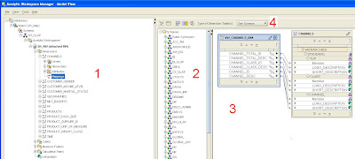
The Mapping Editor
The mapping editor is laid is comprised of four main areas:

In the following sections we will look at how to use the mapping editor to manage different schema layouts to model different types of dimensions and hierarchies.
Types of Dimension Source Tables/Views
Firstly, a quick best practice tip. Personally, I always find it useful to map to views rather than directly to tables. This provides more control over the data passed into the data loader (which can be useful for testing), especially when trying to perform incremental updates from a fact table. But we will look at this in more detail when reviewing processes for designing and building cubes.
Star
A star schema provides one table or view with columns containing member id's representing all levels of a hierarchy for each dimension. Each row in the table specifies a branch in the hierarchy. Additional columns identify additional attributes for each level, such as long and short descriptions. In the case of a time dimension, additional attributes will be required to provide information on end date and time span for each level.
Where a hierarchy is unbalanced and contains skip-levels, or is ragged, or is a combination of both, some rows may contain blank entries in specific columns.
OLAP dimension member ids must be unique within a level, which is normal in relational models, but they may also need to be unique across levels as well. In fact most people forget or try to ignore this requirement and often hit problems later when loading data into their cubes. OLAP stores dimension members as a single continuous list of ids. If your source keys are not unique across levels then you must take the option of generating surrogate keys as stated in the previous workshop.
Enabling the surrogate key option appends the level name to the member id, which should then guarantee uniqueness. However, this is only possible with value-based hierarchies. If your dimension requires a value based hierarchy you must use natural keys.
In summary:

The steps for using a star schema are:
The Mapping Editor allows mapping from the source table to the member and attributes at each level. Each attribute is shown as a separate entry in the dimension object in the editor. The editor will not allow mappings from more than one column to each element, although AWM 11g removes the restriction by allowing simple transformations to be performed during the data loading process.
 Here is an example of a completed mapping for the Product dimension. Note the long and short description attributes share the same source (so it is possible to map a source column to multiple target attributes).

Some query tools will differentiate between long and short descriptions. For example both Discoverer and the OLAP Spreadsheet Addin for Excel will use short descriptions for dimensions used as column headers and long descriptions when the dimension is used in the page or row edge.
If you do not provide a long and./or short description the data loader will default to using the dimension key to populate these attributes.
Snowflake
A snowflake schema provides separate tables or views for each levels of a hierarchy. Each row in the table specifies a level in the hierarchy with an additional column to link to each parent across the various hierarchies. The same basic requirements apply as for star schemas in terms of uniqueness.
Mapping a Snowflake Based Schema

The steps for using a snowflake schema are:
Dimension Objects used in the Mapping
The mapping editor has to be switched to “Snowflake” mode using the pulldown selection dialog at the top of the editor. The mapping canvas will then change to allow you to map each member, its parent and associated attributes at each level.

As with the Star schema mapping process, the snowflake mapping editor will not allow mappings from more than one column to each element i.e., map from a single source table or view per level. Here is a completed snowflake mapping:

Collection of Tables
The basic snowflake schema can be taken a stage further by moving the various attributes, such as descriptions etc, to separate tables. This follows a more 3NF approach to data storage and although it looks more complicated it can easily be managed within AWM's mapping editor.
Mapping a Collection Based Schema

In this format natural or surrogate keys can still be used within the dimension. To map a collection of tables as described above the mapping editor needs to be switched to “Other” mode.

When mapping the tables to the dimension, the normal rules still apply. The Mapping Editor only allows mapping to member, parent for dim values and member, value for attributes at each level. It will not allow mappings from more than one column to each element, but you can map from an arbitrary set of source tables and/or views, which have member and value columns.
Value Based (Parent Child)
This is probably the most simple type of relationship to manage from a mapping perspective. Likely sources for this type of mapping are other AWs, where the source data is from an OLAP enabled SQL view, or another multi-dimensional engine.
The source for this type of relationship is normally a two-column table that provides the key and the parent for each child. Other columns are used to provide additional attributes.

In this case, natural keys must be used to define the dimension, since there are no level identifiers that can be used to construct the surrogate key. In this scenario it is possible to use any of the mapping editor options (star, snowflake, or other) to construct the mapping.

Things to remember when designing a parent-child/value based hierarchy. Firstly, there are no levels, therefore, certain calculations, such as share, are not possible. A parent-child hierarchy cannot be used in the partition statement of a cube because there is no level identifier to act as the partition key.
However, it is possible to provide a pseudo level identified by creating a level attribute. This allows users to create selections using the attribute in the normal way. In some cases, a value based hierarchy may be the only way to manage an unbalanced hierarchy, where not all branches have the same number of dimension members).
Flat List
Another version of the parent-child/value based hierarchy is the flat-list dimension. In this scenario, the dimension has no hierarchies and is simply a flat list of dimension members. Personally, I would not recommend building this type of dimension simply because there is no top level. This makes it difficult for business users to pivot the dimension out of the query since they have to pin the dimension to a specific member when it is hidden. This can make the query process more complicated for business users to understand.
In most cases I would suggest that a flat list hierarchy where no top level is possible is a likely candidate for migration to a series of measures within a cube. This is something you should seriously consider before creating a flat list dimension.
The dimension itself can have a hierarchy based on a single level. This provides the flexibility to use either surrogate or natural keys. If the dimension is designed with no levels and no hierarchy then only natural keys are available.
Skip, Ragged and Ragged-Skip Level Hiearchies
Ragged is a special form of skip. The diagram below shows the various scenarios that can be found in many dimensions. It is highly likely that at least one dimension in a data model will have one or all of these scenarios.

The question is how can such a structure be represented within a relational table?
Skip
Using an across format structure, where a skip level occurs one or more columns are left blank within a specific row. However, within a skip level there is a common leaf node that denotes the lowest level of the hierarchy. From the leaf node to the top level, certain columns that relate to parents of the leaf node are left blank. As shown below (in this case the ID columns are not shown but follow the same pattern)

This type of layout is difficult, if not possible, for most SQL based query tools to manage. However, recent additions to the SQL language has allowed skip-level hierarchies to be partially managed using normal query methods. However, it is only possible to skip one level within a single hierarchy. Fortunately, OLAP does not enforce this constraint.
To map this type of hierarchy use a normal star schema approach. The OLAP engine will manage the complexity of the relationships for you.
Ragged
For a ragged hierarchy, the leaf node will occur at any or all-intervening levels within a hierarchy. Again null values will appear in certain columns within each row.

When defining a ragged hierarchy within a dimension wse natural keys and create a level-based hierarchy(ies). Within the dimension-mapping editor map the source table as a star. But for the cube mapping the fact table requires a little more work. It is necessary to map the key for the ragged dimension to all levels in the dimension, which have leaf values (or, to be safe, map to all levels). This is shown below

Ragged Skip Level
In this scenario, looking at the image at the start of this sectio, we can see the leaves are not always at lowest level; there are some intervening nulls However, this simply a combination of the two types of hierarchies we have already reviewed. The source table would look something like this:

In this scenario the same rules apply as before:
In the next posting in this series we will consider how to design and create cubes.
At the end of the last workshop we had defined a simple time dimension and examined the various components that make up a dimension:
- Levels
- Hierarchies
- Attributes
Most dimensions will have at least one hierarchy, but Oracle OLAP does also support completely flat dimensions where no hierarchy exists. Although this is rare it does occur in some cases, but it is always wise to have an “All Members” level for these types of dimensions as this will allow business users to pivot these types of dimensions out of their query by selecting that top level. Otherwise their queries will always be pinned to a single dimension member within the page dimension.
A hierarchy defines a set of parentage relationships between all or some of a dimension's members:
- Used for rollups of data.
- Used for end-user navigation; e.g., drill-down.

In the first image we have a traditional level based hierarchy where each child has a parent at the next level up in the hierarchy. Although the number of children at each node may, and usually does, differ between nodes. The second image shows another type of level based hierarchy that is some times referred to as a “Skip Level” hierarchy. This is where a leaf node links to a higher-level parent above its next most obvious level. Oracle database can support skip-level relationships within relational hierarchies, however, this is limited to skipping to only one specific level. Oracle OLAP is able to support skip-levels across multiple levels, as seen here:

Oracle OLAP is able to manage these types of relationships quickly and easily because all types of hierarchies are effectively stored as parent-child relationships. A derivation of the skip-level hierarchy is the “Ragged” hierarchy. This is where leaf-nodes are located at different levels within the hierarchy. Obviously this can have an impact on the data loading and aggregation plans, however, Oracle OLAP is more than capable of handling this type of scenario in just the same way as any other level based hierarchy.

Of course you can combine some of these structures to create more complicated relationships such as a “Ragged-Skip” level hierarchy. These more complex structures are also supported.
The last type of hierarchy shown above is a simple flat hierarchy, which as explained earlier may or may not be an ideal type of dimension to model depending on how your business users plan to build queries. In all these cases, the hierarchy is defined based on levels.
One type of hierarchy not shown, but which is supported Oracle OLAP, is “Value” based hierarchies, of which the typical Employee/HR table is the most common example. This type of hierarchy contains no levels and is dealt with as a pure parent-child relationship. In this case the level names are converted into attributes to help business users define the queries.
Across all these types of hierarchies there are some simple rules that need to be followed. It is recommended you create at least one top level on each of your hierarchies. Although some types of dimensions, such as time, will require multiple top levels such as Years.

What you cannot do is have a child owned by multiple parents within the same hierarchy as shown below. In this case, you would need to create two separate hierarchies to manage the relationships separately.

The interesting part here, is the basic design of the dimension and its related levels, hierarchies and attributes is largely consistent across all these different types of structures. The only real different is between level and value-based relationships where value-based dimensions do not contain levels. Fortunately, the dimension loading routines manage these types of dimension structures transparently.
The next step, having defined our dimensions and their associated hierarchies, is to map the source data to the actual dimension itself. To help with this process, and to accommodate some of these more complex relationships, the AWM Mapping Editor allows for three types of source data:
- Star format source table
- Snowflake collection of source tables
- Other
The Mapping Editor
The mapping editor is laid is comprised of four main areas:

- 1 – The mapping editor is launched from the main navigator. There is a mapping editor for each dimension and each cube.
- 2 – Schema List: lists the available tables, views and synonyms where the owner of the AW has been granted SELECT privilege.
- 3 – The mapping Canvas: dragging tables views and.or synonym on to the mapping canvas makes it available for use within a mapping.
- 4 – Mapping Control: Controls the type of layout, which includes:
- Star schema
- Snowflake schema
- Other

In the following sections we will look at how to use the mapping editor to manage different schema layouts to model different types of dimensions and hierarchies.
Types of Dimension Source Tables/Views
Firstly, a quick best practice tip. Personally, I always find it useful to map to views rather than directly to tables. This provides more control over the data passed into the data loader (which can be useful for testing), especially when trying to perform incremental updates from a fact table. But we will look at this in more detail when reviewing processes for designing and building cubes.
Star
A star schema provides one table or view with columns containing member id's representing all levels of a hierarchy for each dimension. Each row in the table specifies a branch in the hierarchy. Additional columns identify additional attributes for each level, such as long and short descriptions. In the case of a time dimension, additional attributes will be required to provide information on end date and time span for each level.
Where a hierarchy is unbalanced and contains skip-levels, or is ragged, or is a combination of both, some rows may contain blank entries in specific columns.
OLAP dimension member ids must be unique within a level, which is normal in relational models, but they may also need to be unique across levels as well. In fact most people forget or try to ignore this requirement and often hit problems later when loading data into their cubes. OLAP stores dimension members as a single continuous list of ids. If your source keys are not unique across levels then you must take the option of generating surrogate keys as stated in the previous workshop.
Enabling the surrogate key option appends the level name to the member id, which should then guarantee uniqueness. However, this is only possible with value-based hierarchies. If your dimension requires a value based hierarchy you must use natural keys.
In summary:
- Natural keys:
- Created in the AW as is from the source table or view (except numeric, dates become text).
- If source table had months 1, 2, 3 then the AW dimension values would be '1', '2', '3'.
- Surrogate keys:
- The level name is prefixed to the source table or view id value.
- If source table had months 1, 2, 3 then the AW dimension values would be 'MONTH_1', 'MONTH_2', 'MONTH_3'

The steps for using a star schema are:
- Use natural or surrogate keys allowed
- Must use surrogate keys if dimension values are not unique across levels.
- Define levels and a level-based hierarchy.
- In the mapping editor choose Star Schema as the Type of Dimension Table(s).
The Mapping Editor allows mapping from the source table to the member and attributes at each level. Each attribute is shown as a separate entry in the dimension object in the editor. The editor will not allow mappings from more than one column to each element, although AWM 11g removes the restriction by allowing simple transformations to be performed during the data loading process.
 Here is an example of a completed mapping for the Product dimension. Note the long and short description attributes share the same source (so it is possible to map a source column to multiple target attributes).
Some query tools will differentiate between long and short descriptions. For example both Discoverer and the OLAP Spreadsheet Addin for Excel will use short descriptions for dimensions used as column headers and long descriptions when the dimension is used in the page or row edge.
If you do not provide a long and./or short description the data loader will default to using the dimension key to populate these attributes.
Snowflake
A snowflake schema provides separate tables or views for each levels of a hierarchy. Each row in the table specifies a level in the hierarchy with an additional column to link to each parent across the various hierarchies. The same basic requirements apply as for star schemas in terms of uniqueness.
Mapping a Snowflake Based Schema

The steps for using a snowflake schema are:
- Natural or surrogate keys allowed
- Must use surrogate keys if dim values are not unique across levels.
- Define levels and a level-based hierarchy.
- Choose Snowflake schema as the Type of Dimension Table(s).
Dimension Objects used in the Mapping
The mapping editor has to be switched to “Snowflake” mode using the pulldown selection dialog at the top of the editor. The mapping canvas will then change to allow you to map each member, its parent and associated attributes at each level.

As with the Star schema mapping process, the snowflake mapping editor will not allow mappings from more than one column to each element i.e., map from a single source table or view per level. Here is a completed snowflake mapping:

Collection of Tables
The basic snowflake schema can be taken a stage further by moving the various attributes, such as descriptions etc, to separate tables. This follows a more 3NF approach to data storage and although it looks more complicated it can easily be managed within AWM's mapping editor.
Mapping a Collection Based Schema

In this format natural or surrogate keys can still be used within the dimension. To map a collection of tables as described above the mapping editor needs to be switched to “Other” mode.

When mapping the tables to the dimension, the normal rules still apply. The Mapping Editor only allows mapping to member, parent for dim values and member, value for attributes at each level. It will not allow mappings from more than one column to each element, but you can map from an arbitrary set of source tables and/or views, which have member and value columns.
Value Based (Parent Child)
This is probably the most simple type of relationship to manage from a mapping perspective. Likely sources for this type of mapping are other AWs, where the source data is from an OLAP enabled SQL view, or another multi-dimensional engine.
The source for this type of relationship is normally a two-column table that provides the key and the parent for each child. Other columns are used to provide additional attributes.

In this case, natural keys must be used to define the dimension, since there are no level identifiers that can be used to construct the surrogate key. In this scenario it is possible to use any of the mapping editor options (star, snowflake, or other) to construct the mapping.

Things to remember when designing a parent-child/value based hierarchy. Firstly, there are no levels, therefore, certain calculations, such as share, are not possible. A parent-child hierarchy cannot be used in the partition statement of a cube because there is no level identifier to act as the partition key.
However, it is possible to provide a pseudo level identified by creating a level attribute. This allows users to create selections using the attribute in the normal way. In some cases, a value based hierarchy may be the only way to manage an unbalanced hierarchy, where not all branches have the same number of dimension members).
Flat List
Another version of the parent-child/value based hierarchy is the flat-list dimension. In this scenario, the dimension has no hierarchies and is simply a flat list of dimension members. Personally, I would not recommend building this type of dimension simply because there is no top level. This makes it difficult for business users to pivot the dimension out of the query since they have to pin the dimension to a specific member when it is hidden. This can make the query process more complicated for business users to understand.
In most cases I would suggest that a flat list hierarchy where no top level is possible is a likely candidate for migration to a series of measures within a cube. This is something you should seriously consider before creating a flat list dimension.
The dimension itself can have a hierarchy based on a single level. This provides the flexibility to use either surrogate or natural keys. If the dimension is designed with no levels and no hierarchy then only natural keys are available.
Skip, Ragged and Ragged-Skip Level Hiearchies
Ragged is a special form of skip. The diagram below shows the various scenarios that can be found in many dimensions. It is highly likely that at least one dimension in a data model will have one or all of these scenarios.

The question is how can such a structure be represented within a relational table?
Skip
Using an across format structure, where a skip level occurs one or more columns are left blank within a specific row. However, within a skip level there is a common leaf node that denotes the lowest level of the hierarchy. From the leaf node to the top level, certain columns that relate to parents of the leaf node are left blank. As shown below (in this case the ID columns are not shown but follow the same pattern)

This type of layout is difficult, if not possible, for most SQL based query tools to manage. However, recent additions to the SQL language has allowed skip-level hierarchies to be partially managed using normal query methods. However, it is only possible to skip one level within a single hierarchy. Fortunately, OLAP does not enforce this constraint.
To map this type of hierarchy use a normal star schema approach. The OLAP engine will manage the complexity of the relationships for you.
Ragged
For a ragged hierarchy, the leaf node will occur at any or all-intervening levels within a hierarchy. Again null values will appear in certain columns within each row.

When defining a ragged hierarchy within a dimension wse natural keys and create a level-based hierarchy(ies). Within the dimension-mapping editor map the source table as a star. But for the cube mapping the fact table requires a little more work. It is necessary to map the key for the ragged dimension to all levels in the dimension, which have leaf values (or, to be safe, map to all levels). This is shown below

Ragged Skip Level
In this scenario, looking at the image at the start of this sectio, we can see the leaves are not always at lowest level; there are some intervening nulls However, this simply a combination of the two types of hierarchies we have already reviewed. The source table would look something like this:

In this scenario the same rules apply as before:
- Use natural keys, level-based hierarchy(ies).
- Map as a star.
- When map the fact table, map its key to all levels in the dimension which have leaf values.
In the next posting in this series we will consider how to design and create cubes.
Subscribe to:
Posts (Atom)


