Another new tutorial has been added to the Oracle OLAP home page on OTN.
This tutorial is titled 'Oracle OLAP 11g: Setting Up Cube Materialized Views for Query Rewrite'
The tutorial describes how to enable cubes as Cube Materialized Views, and how to enable and troubleshoot Query Rewrite using Analytic Workspace Manager 11.1.0.7. It is intended as a quickstart for intermediate developers.
Showing posts with label Workshop. Show all posts
Showing posts with label Workshop. Show all posts
Tuesday, December 16, 2008

Tuesday, November 25, 2008
New 11g OLAP tutorial posted onto OTN
A new tutorial has been added to OTN.
The tutorial is aimed at newcomers to Oracle OLAP and is a guide to creating and populating an 11g OLAP cube.
This is perfect for people who are looking for a gentle introduction to using the Analytic Workspace Manager OLAP administration tool and understand the basic steps in building an 11g OLAP cube.
The tutorial is aimed at newcomers to Oracle OLAP and is a guide to creating and populating an 11g OLAP cube.
This is perfect for people who are looking for a gentle introduction to using the Analytic Workspace Manager OLAP administration tool and understand the basic steps in building an 11g OLAP cube.
Thursday, March 27, 2008
Creating A Calculated Measure Cube - IOGALFF
(Firstly, this is information relates only to OLAP 10gR2. There are a number of changes within OLAP11gR1 and the following scenario has not been tested with 11g)
When you venture into most supermarkets today, somewhere on one of the many isles there will be a BOGOF – buy one get one free. Well how about an OLAP offer: “IOGALFF” – install one get at least fourteen free. I admit it is not quite as catchy as the original, but the benefits are huge and it has the result of making life so much easier.One of the more interesting challenges of using Analytic Workspace Manager (and also OWB) relates to managing all the calculated measures within a cube. Every measure should really be accompanied by a standard set of calculated measures such as:
- Current Period
- Last Year
- Last Year %
- Prior Period
- Prior Period %
- Year to Date
- Year to Date Last Year
- Year to Date Last Year %
- Quarter to Date
- Quarter to Date Last Year
- Quarter to Date Last Year %
- 3-Month Moving Average
- 6-Month Moving Average
- 12-Month Moving Average
- Dimension “A” Share of All Members
- Dimension “A” Share of Parent
Its is the addition of these types of measures that adds real value to the your BI application. As I have stated many times before: business users are not interested in looking at data from base measures, typically they are more interested in trends based on the prior period or prior year, share of revenue, moving averages and so on. This adds a lot of work for the cube designer as they need to add at least 14 calculated measures for each base measure as well as two additional calculated share measures for each dimension associated with each cube.
Which adds up to a lot of measures and manually creating all these measure is likely to take a considerable amount of time. If we take the command schema sample that is shipped with BI10g, this contains 5 base measures (costs, quantity, revenue, margin, price) with 4 dimensions (channel, geography, product, time), which translates to
5 * 14 calculated measures
+
5 * 3 (dimensions - channel, geography, product) * 2 calculated share measures
= 100 calculated measures.
As I said, it is very easy to generate a lot of calculated measures.
So is there a more intelligent way of managing calculated measures? What is the quickest way to add all these additional calculations to a cube? One way is to use the Excel Accelerator to add the calculated measures to your AW. It is relatively easy to use and allows you to use normal Excel tools such as cut & paste to quickly create all the calculations you could ever need. You can download the Excel Accelerator from the OLAP OTN Home Page, or by clicking here. Look for these links:
Creating OLAP Calculations using Excel
Creating OLAP Calculations using Exce Readme
During a recent POC, we used a more interesting approach that takes the use of customer calculations to a new level. In many ways this goes back to the various techniques we used when creating Express databases for use with Sales Analyzer to make life easier for both administrators and users. The approach is quite simple – use and additional dimension to define the type of calculation you want to execute and link this to a DML program to return the required results. The list of calculated measures listed above are converted into dimension members, which provides another way to slice, dice and pivot the data. As you can see here, the dimension member that identifies the type of calculation is in the row edge with the measure in the column edge. In this way, only one calculation is required which is used across all the available measures.

What this means is: by installing one simple (well, everything is relative) calculated measure you can get upto fourteen additional calculations for free. Hence the acronym “IOGALFF” – install one get at least fourteen free.
How is all this managed? There are five basic steps to creating this type of reporting solution:
- Create a new dimension to control the types of calculations returned
- Add some additional attributes to the time dimension to help manage some of the time series arguments for specific calculations
- Create an OLAP DML program to return the data
- Create a new cube that includes the new calculation type dimension and add a calculated measure that calls the OLAP DML program to return the required data
- Create a SQL View over the cube
Step 1 – Creating the new Time View dimension
I have called the dimension containing the list of calculated members, Time View (mainly because the majority of the calculations are time based but may be a better name would be "measure view" ?). The Time View dimension has one level and one hierarchy with three attributes:
- Long Label
- Short Label
- Default sort order

The source data looks like this:

With the source table definition as follows:
CREATE TABLE TIME_VIEW
(TIME_VIEW_ID VARCHAR2(2 BYTE),
TIME_VIEW_DESC VARCHAR2(35 BYTE),
SORT_ORDER NUMBER(*,0));
And the view definition as follows:
CREATE OR REPLACE FORCE VIEW VW_TIME_VIEW AS
SELECT
TIME_VIEW_ID
, TIME_VIEW_DESC
, SORT_ORDER
FROM TIME_VIEW
ORDER BY SORT_ORDER;
To populate the base table the following commands are used:
INSERT INTO TIME_VIEW VALUES ('1', 'Current Period', '1')
INSERT INTO TIME_VIEW VALUES ('2', 'Last Year', '2')
INSERT INTO TIME_VIEW VALUES ('3', 'Last Year %', '3')
INSERT INTO TIME_VIEW VALUES ('4', 'Prior Period', '4')
INSERT INTO TIME_VIEW VALUES ('5', 'Prior Period %', '5')
INSERT INTO TIME_VIEW VALUES ('6', 'Year To Date', '6')
INSERT INTO TIME_VIEW VALUES ('7', 'Year To Date Last Year', '7')
INSERT INTO TIME_VIEW VALUES ('8', 'Year To Date Last Year %', '8')
INSERT INTO TIME_VIEW VALUES ('9', 'Quarter To Date', '9')
INSERT INTO TIME_VIEW VALUES ('10', 'Quarter To Date Last Year', '10')
INSERT INTO TIME_VIEW VALUES ('11', 'Quarter To Date Last Year %', '11')
INSERT INTO TIME_VIEW VALUES ('12', '3-Month Moving Average', '12')
INSERT INTO TIME_VIEW VALUES ('13', '6-Month Moving Average', '13')
INSERT INTO TIME_VIEW VALUES ('14', '12-Month Moving Average', '14')
After this, the next set of values depends on the dimensions within your data model. For my model, I have three additional dimensions that I want to analyze: Channel, Product and Customer. For each of these dimensions I want to see the % share of each member in relation to the value for all members (i.e. the top level) and the shared based on the parent value. To enable these calculations I add the following lines to the TIME_VIEW table:
INSERT INTO TIME_VIEW VALUES ('15', ' Product Share of All Products', '15')
INSERT INTO TIME_VIEW VALUES ('16', ' Product Share of Parent', '16')
INSERT INTO TIME_VIEW VALUES ('17', ' Channel Share of All Channels', '17')
INSERT INTO TIME_VIEW VALUES ('18', ' Channel Share of Parent', '18')
INSERT INTO TIME_VIEW VALUES ('19', ' Customer Share of All Customers', '19')
INSERT INTO TIME_VIEW VALUES ('20', ' Customer Share of Parent', '20')
(Obviously, these additional share calculations are not really related to time, so using the name Time View is sort of confusing and in hindsight the term Measure View would have been a better name for the dimension). Once the table has been defined, it can be mapped in AWM to create the dimension mapping (in this case I am using a view over the source

The last part of this step is to then load the members into the dimension using the dimension data load wizard or via the SQL command line using a load script. The result should look like this when you view the members using the Dimension Data Viewer:

As can be seen here, there are fourteen base calculations that can be applied to any model, plus the additional share calculations that are based on the dimensions within the source cube. Hence the title “IOGALFF” – install one get fourteen free. In reality it is more like: install one and as many calculations as you like or need, but that translates to “IOGASMAYNORL” which does not really role off the tongue.
Step 2 – Updating the Time Dimension with new Attributes.
To make the program that delivers all these calculated measures as simple as possible a number of attributes are added to the time dimension:
- Lag Prior Year
- At the Year level this equates to 1
- At the Quarter level this equates to 4
- At the Month level this equates to 12
- At the Day level it is the number of days in the year (365 or 366)
- Parent Quarter
- This is the quarter for each time period and used as the reset trigger for the cumulative totals
- Parent Year
- This is the year for each time period and used as the reset trigger for the cumulative totals

The information for the two parent attributes is taken from existing columns within the source data since this information already exists and the Lag Prior Year is a simple hard-coded value apart from the day level where the timespan value for the year is used to cope with leap years. Therefore, all the information for these three attributes should be readily available within your source data, especially if you are using the OWB Time Wizard to create your time dimension. Obviously using a view over the source table for the mapping within AWM makes adding this information relatively trivial.
Step 3 – Create the OLAP DML Calculation Program.
The new OLAP DML program, called TIME_VIEW_PRG (again feel free to change the name of program if you want), takes two arguments:
- The cube.measure_name for the base measure, in this case SALES_M1, which is the Revenue measure in the SALES cube.
- The identifier for the calculated measure within the REPORT_CUBE cube, which in this case is M1_PRG (this is explained in more detail in the next section)
DEFINE TIME_VIEW_PRG PROGRAM DECIMAL
argument T_MEASURE text " Full measure name including cube name
argument T_MEASURE_ID text " Measure name
variable T_FORM text " Name of the formula
variable T_TIME_VIEW text " Value of TIME_VIEW dimension
variable D_RETURN decimal " Return value
trap on ALLDONE noprint
T_TIME_VIEW = TIME_VIEW
T_FORM = joinchars('REPORT_CUBE_', T_MEASURE_ID)
switch T_TIME_VIEW
do
case 'VL1_1':
D_RETURN = &T_MEASURE
break
case 'VL1_2': "LY
D_RETURN = lag(&T_FORM(TIME_VIEW 'VL1_1'), TIMES_LAG_PRIOR_YEAR, TIMES, LEVELREL TIMES_LEVELREL)
break
case 'VL1_3': "LY%
D_RETURN = lagpct(&T_FORM(TIME_VIEW 'VL1_1'), TIMES_LAG_PRIOR_YEAR, TIMES, LEVELREL TIMES_LEVELREL)
break
case 'VL1_4': "PP
D_RETURN = lag(&T_FORM(TIME_VIEW 'VL1_1'), 1, TIMES, LEVELREL TIMES_LEVELREL)
break
case 'VL1_5': "PP%
D_RETURN = lagpct(&T_FORM(TIME_VIEW 'VL1_1'), 1, TIMES, LEVELREL TIMES_LEVELREL)
break
case 'VL1_6': "YTD
if TIMES_LEVELREL EQ 'YEAR'
then D_RETURN = &T_FORM(TIME_VIEW 'VL1_1')
else D_RETURN = cumsum(&T_FORM(TIME_VIEW 'VL1_1'), TIMES, TIMES_PARENT_YEAR)
break
case 'VL1_7': "YTD LY
if TIMES_LEVELREL EQ 'YEAR'
then D_RETURN = lag(&T_FORM(TIME_VIEW 'VL1_1'), TIMES_LAG_PRIOR_YEAR, TIMES, LEVELREL TIMES_LEVELREL)
else D_RETURN = cumsum(lag(&T_FORM(TIME_VIEW 'VL1_1'), TIMES_LAG_PRIOR_YEAR, TIMES, LEVELREL TIMES_LEVELREL), TIMES, TIMES_PARENT_YEAR)
break
case 'VL1_8': "YTD LY%
D_RETURN = (&T_FORM(TIME_VIEW 'VL1_6')-cumsum(lag(&T_FORM(TIME_VIEW 'VL1_1'), TIMES_LAG_PRIOR_YEAR, TIMES, LEVELREL TIMES_LEVELREL), TIMES, TIMES_PARENT_YEAR))/cumsum(lag(&T_FORM(TIME_VIEW 'VL1_1'), TIMES_LAG_PRIOR_YEAR, TIMES, LEVELREL TIMES_LEVELREL), TIMES, TIMES_PARENT_YEAR)
break
case 'VL1_9': "QTD
if TIMES_LEVELREL EQ 'YEAR'
then D_RETURN = NA
else if TIMES_LEVELREL EQ 'QUARTER'
then D_RETURN = &T_FORM(TIME_VIEW 'VL1_1')
else if TIMES_LEVELREL EQ 'MONTH'
then D_RETURN = cumsum(&T_FORM(TIME_VIEW 'VL1_1'), TIMES, TIMES_PARENT_QUARTER)
else if TIMES_LEVELREL EQ 'DAY'
then D_RETURN = cumsum(&T_FORM(TIME_VIEW 'VL1_1'), TIMES, TIMES_PARENT_QUARTER)
else D_RETURN = NA
break
case 'VL1_10': "QTD LY
if TIMES_LEVELREL EQ 'YEAR'
then D_RETURN = NA
else if TIMES_LEVELREL EQ 'QUARTER'
then D_RETURN = cumsum(lag(&T_FORM(TIME_VIEW 'VL1_1'), TIMES_LAG_PRIOR_YEAR, TIMES, LEVELREL TIMES_LEVELREL), TIMES, TIMES_PARENT_QUARTER)
else if TIMES_LEVELREL EQ 'MONTH'
then D_RETURN = cumsum(lag(&T_FORM(TIME_VIEW 'VL1_1'), TIMES_LAG_PRIOR_YEAR, TIMES, LEVELREL TIMES_LEVELREL), TIMES, TIMES_PARENT_QUARTER)
else if TIMES_LEVELREL EQ 'DAY'
then D_RETURN = cumsum(lag(&T_FORM(TIME_VIEW 'VL1_1'), TIMES_LAG_PRIOR_YEAR, TIMES, LEVELREL TIMES_LEVELREL), TIMES, TIMES_PARENT_QUARTER)
break
case 'VL1_11': "QTD LY%
if TIMES_LEVELREL EQ 'YEAR'
then D_RETURN = NA
else if TIMES_LEVELREL EQ 'QUARTER'
then D_RETURN = (&T_FORM(TIME_VIEW 'VL1_9')-cumsum(lag(&T_FORM(TIME_VIEW 'VL1_1'), TIMES_LAG_PRIOR_YEAR, TIMES, LEVELREL TIMES_LEVELREL), TIMES, TIMES_PARENT_QUARTER))/cumsum(lag(&T_FORM(TIME_VIEW 'VL1_1'), TIMES_LAG_PRIOR_YEAR, TIMES, LEVELREL TIMES_LEVELREL), TIMES, TIMES_PARENT_QUARTER)
else if TIMES_LEVELREL EQ 'MONTH'
then D_RETURN = (&T_FORM(TIME_VIEW 'VL1_9')-cumsum(lag(&T_FORM(TIME_VIEW 'VL1_1'), TIMES_LAG_PRIOR_YEAR, TIMES, LEVELREL TIMES_LEVELREL), TIMES, TIMES_PARENT_QUARTER))/cumsum(lag(&T_FORM(TIME_VIEW 'VL1_1'), TIMES_LAG_PRIOR_YEAR, TIMES, LEVELREL TIMES_LEVELREL), TIMES, TIMES_PARENT_QUARTER)
else if TIMES_LEVELREL EQ 'DAY'
then D_RETURN = (&T_FORM(TIME_VIEW 'VL1_9')-cumsum(lag(&T_FORM(TIME_VIEW 'VL1_1'), TIMES_LAG_PRIOR_YEAR, TIMES, LEVELREL TIMES_LEVELREL), TIMES, TIMES_PARENT_QUARTER))/cumsum(lag(&T_FORM(TIME_VIEW 'VL1_1'), TIMES_LAG_PRIOR_YEAR, TIMES, LEVELREL TIMES_LEVELREL), TIMES, TIMES_PARENT_QUARTER)
break
case 'VL1_12': "3MMA
if TIMES_LEVELREL eq 'MONTH'
then D_RETURN = MOVINGAVERAGE(&T_FORM(TIME_VIEW 'VL1_1'), -2, 0, 1, TIMES, LEVELREL TIMES_LEVELREL)
else D_RETURN = NA
break
case 'VL1_13': "6MMA
if TIMES_LEVELREL eq 'MONTH'
then D_RETURN = MOVINGAVERAGE(&T_FORM(TIME_VIEW 'VL1_1'), -5, 0, 1, TIMES, LEVELREL TIMES_LEVELREL)
else D_RETURN = NA
break
case 'VL1_14': "12MMA
if TIMES_LEVELREL eq 'MONTH'
then D_RETURN = MOVINGAVERAGE(&T_FORM(TIME_VIEW 'VL1_1'), -11, 0, 1, TIMES, LEVELREL TIMES_LEVELREL)
else D_RETURN = NA
break
case 'VL1_15': "Product Share of All Products
D_RETURN = &T_FORM(TIME_VIEW 'VL1_1')/&T_FORM(TIME_VIEW 'VL1_1', PRODUCTS limit(PRODUCTS to TOPANCESTORS using PRODUCTS_PARENTREL)
break
case 'VL1_16': "Product Share of Parent
D_RETURN = &T_FORM(TIME_VIEW 'VL1_1')/&T_FORM(TIME_VIEW 'VL1_1', PRODUCTS PRODUCTS_PARENTREL)
break
case 'VL1_17': "Customers Share of All Customers
D_RETURN = &T_FORM(TIME_VIEW 'VL1_1')/&T_FORM(TIME_VIEW 'VL1_1', CUSTOMERS limit(CUSTOMERS to TOPANCESTORS using CUSTOMERS_PARENTREL)
break
case 'VL1_18': "Customers Share of Parent
D_RETURN = &T_FORM(TIME_VIEW 'VL1_1')/&T_FORM(TIME_VIEW 'VL1_1', CUSTOMERS CUSTOMERS_PARENTREL)
break
case 'VL1_19': "Channels Share of All Channels
D_RETURN = &T_FORM(TIME_VIEW 'VL1_1')/&T_FORM(TIME_VIEW 'VL1_1', CHANNELS limit(CHANNELS to TOPANCESTORS using CHANNELS_PARENTREL)
break
case 'VL1_20': "Channels Share of Parent
D_RETURN = &T_FORM(TIME_VIEW 'VL1_1')/&T_FORM(TIME_VIEW 'VL1_1', CHANNELS CHANNELS_PARENTREL)
break
doend
ALLDONE:
return D_RETURN
END
In simple terms, the program checks to see which member of the dimension TIME_VIEW is being requested and then executes the correct OLAP function to return the required data. At the moment this has only been tested on a Julian calendar hierarchy but I am doing some more testing over the next few weeks for other types of hierarchies. Some of the measures are dependant on the level within the Time dimension, so you may need to change references to specific level names etc if you want to reuse this program code. For example:
if TIMES_LEVELREL EQ 'YEAR'
My time dimension has levels; Year, Quarter, Month, and Day. In some cases it is necessary to change the processing depending the level, for example:
if TIMES_LEVELREL EQ 'YEAR'
then D_RETURN = NA
else if TIMES_LEVELREL EQ 'QUARTER'
then D_RETURN = &T_FORM(TIME_VIEW 'VL1_1')
else if TIMES_LEVELREL EQ 'MONTH'
then D_RETURN = cumsum(&T_FORM(TIME_VIEW 'VL1_1'), TIMES, TIMES_PARENT_QUARTER)
else if TIMES_LEVELREL EQ 'DAY'
then D_RETURN = cumsum(&T_FORM(TIME_VIEW 'VL1_1'), TIMES, TIMES_PARENT_QUARTER)
else D_RETURN = NA
In this code extract you can see the reference to one of the additional time attributes we added in the previous step, PARENT_QUARTER that is used by the program. All the references within the program are based on Standard Form naming conventions. Therefore, the full standard name for this attribute is TIMES_PARENT_QUARTER since the dimension is called TIMES and the attribute is called PARENT_QUARTER.
For simplicity I created the program in the AW containing the cubes, which is not exactly ideal because if you delete the AW to rebuild it you will lose the program code. Alternatively, you can just create a new AW and add the program to the new AW then modify the ONTTACH program in your data AW to automatically attach the program AW.
Calculations for dimension members VL_15 to VL_20 are provided as examples and would need to be changed to match the dimensions within your own AWs. For each dimension you will need to create two new dimension members within the TIME_VIEW dimension to return the following share calculations:
- Share of based on the top level total, i.e. All Members
- Share based on parent.
case 'VL1_19': "Channels Share of All Channels
D_RETURN = &T_FORM(TIME_VIEW 'VL1_1')/&T_FORM(TIME_VIEW 'VL1_1', CHANNELS limit(CHANNELS to TOPANCESTORS using CHANNELS_PARENTREL)
break
case 'VL1_20': "Channels Share of Parent
D_RETURN = &T_FORM(TIME_VIEW 'VL1_1')/&T_FORM(TIME_VIEW 'VL1_1', CHANNELS CHANNELS_PARENTREL)
break
Step 4 – Creating the New Cube.
In my demo schema I have a cube called SALES and it contains two measures: Revenue (called M1) and Quantity (called M2). The dimensionality for this cube is Time, Channel Product, and Customer.
To provide all the time series and comparative calculations I create a new cube that has the same dimensionality as the SALES cube, with one additional dimension. In this cube the Time View dimension is also used. This reporting cube contains no stored measures, but it does contain custom calculated measures for each measure in the SALES cube, however, each calculated measure will return 14 additional time calculations and 6 share calculations to support the base measure controlled by the dimension TIME_VIEW.

The implementation for the cube is largely irrelevant since no stored measures will be present within the cube, only calculated measures. Therefore, you can if you want either accept the default settings or de-select all the various options.

To add the calculated measures to the cube requires the use of a custom measure XML template. To create a calculated measure to support the measure “Revenue” from the SALES cube you will need to create a custom calculation either using an XML template (email me I can send you a blank template) or use the Excel Calculation Utility that can be downloaded from the OLAP Home Page on OTN to install the two custom calculations.
Once you have added these calculated measures to the REPORT_CUBE, the tree in AWM should look like this:

By selecting each of the calculated measures, the details of each calculation will be displayed within the right-hand panel of AWM. For the first calculated measure linked the Revenue measure in the Sales cube the panel looks like this:

For the second calculated measure linked the Quantity measure in the Sales cube the panel looks like this:

The key part is the line showing the “Expression” (in the XML Template this is the attribute ExpressionText), this defines the call to an OLAP DML program called TIME_VIEW_PRG passing the two required arguments of
ExpressionText="TIME_VIEW_PRG('SALES_M1', 'M1_PRG')”
- The cube.measure_name for the base measure, in this case SALES_M1, which is the Revenue measure in the SALES cube.
- The identifier for the calculated measure within the REPORT_CUBE cube.
- CNS REPORT_CUBE_M1_PRG
- EQ TIME_VIEW_PRG('SALES_M1', 'M1_PRG')
- UPDATE
- COMMIT
- CNS REPORT_CUBE_M2_PRG
- EQ TIME_VIEW_PRG('SALES_M2', 'M2_PRG')
- UPDATE
- COMMIT
If want to do this via the PL/SQL interface then you can do something like this:
EXEC DBMS_AW.EXECUTE('AW ATTACH AW_NAME RW FIRST')
EXEC DBMS_AW.EXECUTE('CNS REPORT_CUBE_M1_PRG')
EXEC DBMS_AW.EXECUTE('EQ TIME_VIEW_PRG(''SALES_M1'', ''M1_PRG'')')
EXEC DBMS_AW.EXECUTE('UPDATE')
EXEC DBMS_AW.EXECUTE('COMMIT')
EXEC DBMS_AW.EXECUTE('CNS REPORT_CUBE_M2_PRG')
EXEC DBMS_AW.EXECUTE('EQ TIME_VIEW_PRG(''SALES_M2'', ''M2_PRG'')')
EXEC DBMS_AW.EXECUTE('UPDATE')
EXEC DBMS_AW.EXECUTE('COMMIT')
EXEC DBMS_AW.EXECUTE('AW DETACH AW_NAME')
Step 4a – Viewing the Data.
Once the calculated measures have been added to the new cube, REPORT_CUBE, the AWM Data Viewer can be launched to check the results:

In the Query Wizard both sets of measures (stored measures and the new calculated measures) are both available for selection. To see the new calculations that are now available we can select both of the Report View measures as shown here.
Once the measures have been selected, the dimension selector will allow us to pick the calculations we want to display from the list of twenty (there are fourteen base calculations that can be applied to any model, plus the additional share calculations that are based on the dimensions within the source cube, in this case six additional share calculations, making twenty calculated measures in total).

The Dimension Viewer shows all the available calculations for this demo schema and the final report is shown below.

Step 5 – Making the Data Available via SQL.
Is there any real point to this post except to show how clever Oracle OLAP can be? In opinion yes, since this technique can be extremely useful when you need to make an OLAP cube visible to SQL based tools. Analytic Workspace Manager 10g has an relational view generator that is available as a plugin and this makes generating the SQL views to support your OLAP cubes a very quick and easy process. But there we know users don’t just want base measures they want lots and lots of calculations as well. When the time comes to create SQL views as the limit on the number of columns within a view is 1000. This may have been increased in 10g/11g, but even so, navigating a cube with that many columns is not easy.
The OLAP View Generator plugin for AWM10gR2 can be downloaded from here, and the associated readme is here.
Using this model, the calculations simply resolve to another dimension, which translates to one additional column in the view as opposed to, at least, 14 additional columns per source measure and in this case 20 additional columns per source measure. Therefore, this approach makes exposing the cube much easier to manage as can be seen here:

As we can see here, all the calculations are contained within the dimension Time View, which simply gets exposed like any other dimension.
Eh voila, install one measure and you can automatically generate fourteen or more additional measures which are guaranteed to bring a smile to the face of any business user.
Friday, March 7, 2008
OLAP Workshop 7 : Creating Calculated Measures
Most data warehouses contain a lot of data but also conversely contain very little information. Many DW teams are content to publish basic facts to their user communities and then leave those communities to fend for themselves in turning data into information. For example, it is not uncommon to see basic measures such as sales, costs, and stock in many data warehouse schemas, but in reality these types of measures are completely useless in themselves. Business users are not interested per se in the value of sales today and this can be seen in the general press as well when reporting key trading periods such as Thanksgiving in the US and Christmas in Europe. Both business and financial communities are both more interested in sales compared to the same time last year, rate of growth of sales, sales compared to forecast. In other words most people are actually interested in calculated measures such as ratios and percentages derived from the base data.
Therefore, the key question for many data warehouse teams is how to create and manage these types of calculations?
In this workshop we will explore some the calculated measures that can be quickly and easily created in your analytic workspace (AW) to enrich its analytic content for end users.
One of the powerful features of the Oracle OLAP technology is the ability to efficiently and easily create business calculations. Oracle OLAP contains a powerful calculation engine that allows you to extend the analytic content of your AW by adding into it some useful business calculations as calculated measures. Some of these business calculations are simple and some of are a lot more involved. However, none are complex from an end-user perspective, although many of them are challenging to traditional relational-only databases. This is especially true when the calculations are numerous, and when many of the queries are ad hoc and unpredictable in nature.
Calculated measures are, as the name suggests, calculated from other measures available in the AW. They are implemented as formulas in the AW; that is, their definition is saved, but no calculated data is stored. The calculations happen at run time when a query requires it. Calculated measures are derived from the contents of other measures, including stored measures as well as measures that are calculated at run time. The calculated measures that you define in the AW are indistinguishable to end users from the stored measures into which data has been loaded and stored in the AW. All measures, according to the dimensional model presented to the end user, are identical. This promotes ease of use by end users.
There is generally a trade-off between precomputing and storing measures in the AW versus calculating them at query time. However, Oracle AWs are very efficient at preserving query performance at very fast levels, even when there are many calculated measures that are resolved dynamically. It is not uncommon for Oracle OLAP customers to implement multidimensional cubes with many hundreds or even thousands of calculated measures and key performance indicators (KPIs), which are calculated at query time from a relatively small number of physically stored and aggregated (or partially aggregated) measures. It is a striking characteristic of AWs in the Oracle database that query performance generally remains consistent even as data volumes and calculation complexity increase.
So how do calculated measures works and what happens when the dimensionality of the source measures does not match exactly?
In the example below a measure called Revenue is a calculated measure based on two other measures: quantity and price. The calculation itself is simple: quantity × price. Notice that the resulting dimensionality of Revenue is inherited from the two measures involved in the calculation. When you use measures with different dimensionality in a calculation, the result always contains the superset of the dimensions of the base measures. The multidimensional data model handles this automatically. You do not have to worry about the possibility that different measures in your AW have different shapes or dimensionality. You specify the calculation rule in the wizard, and the engine automatically resolves the dimensionality. One obvious requirement is that one dimension must be in common for the result to make sense.
In this example, Quantity is dimensioned by Time, Product, and Customer but Unit Price is not dimensioned by Customer. When Oracle OLAP is asked to calculate quantity × price, it uses its knowledge of the dimensional model to automatically handle the calculation of Revenue for all customers, even though there is no separate price stored for each customer. If there is not a separate price for each customer, then there must be a single price for all customers. Price does not vary by customer. As Oracle OLAP performs the calculation quantity × price, it applies the appropriate price for the particular product and time dimension intersections being calculated.

There are two methods for creating a calculated measure
By default both AWM and OWB provide a calculation wizard to help define the most common types of business calculaltions. There are four categories of calculations:


Creating a Share Calculation
The Share template prompts you for the components you need to specify the calculation:
Share Of: A measure or calculated measure that is dimensioned by the Product dimension (in this example)
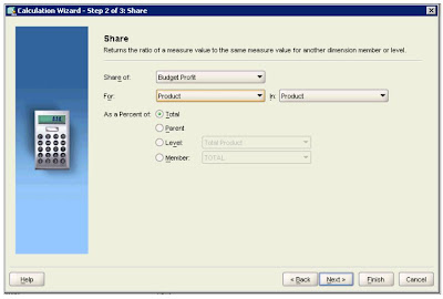
So, as can be seen with this share calculation template it may be necessary to create multiple calculated measures using the same template to provide different results, such as shown below:

This report is showing the Budget Profit base measure and three Share calculations: Share of Product Total, Share of Product Level, and Share of a Product Member (Hardware). Note how the “% of Total,” “% of Level,” and “% of HW ” (hardware) category measures behave differently as the user drills down the product hierarchy. Also note that the third share measure on the report is base-lined to a specific product: the Hardware category. The report shows how Hardware compares to the other categories: Electronics, Peripherals and Accessories, Photo, and Software/Other.
Creating a % Different Prior Period Calculation
Using the “Percent Difference from Prior Period” calculated measure template, you can create a calculated measure that is useful to indicate growth or decline of a business over time. This calculation template is found in the Prior/Future Time Period calculation type folder. This template accepts input for the following items to calculate the percentage difference from a prior period:

In a report this would look like this:
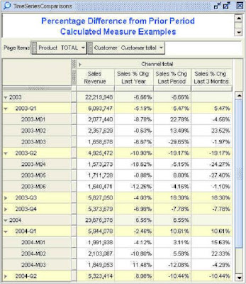
This report contains calculations of a number of alternative percentage differences from prior periods. All the measures automatically handle the situation in which the user needs to drill down into the time dimension and look at time periods at different levels. A single calculated measure in the AW can be used at any level of time, by any query tool, including SQL tools.
Note the following:
Creating a Moving Average Calculation
The Moving Average calculated measure template enables you to create moving averages over any of the measures in your AW. Moving averages are very useful when you analyze volatile data, because they smooth out the peaks and troughs and enable you to more easily visualize the trend in data. In the Moving Average template, you are asked to provide the following input:

Below is a combination graph showing how moving averages can be a useful way of smoothing out volatile data, thus enabling you to see the trends in data more easily.
One line is a moving six-month average, and the other line is a three-month average.

Modifying a Calculated Measure
Existing calculated measures can be edited from within AWM 10g. The descriptions and the calculation details can be changed. To change a calculated measure, click the calculated measure in the Model view. You see the general information displayed on the right. You can:

Managing Calculated Measures
My recommendation is always to create your calculated measures in a separate cube. This helps insulate you from changes to the physical implementation of your base cubes. For example, if you want to change the storage definition for a cube AWM forces you to delete the cube, which if it contains calculated measures means these are also delete and need to be recreated. By keeping your calculated measures in a separate cube it is possible to delete and a rebuild a cube without impacting the calculated measures. Assuming of course you do not change the dimensionality.
There are other ways to resolve this issue (deleting a cube but keeping the calculated measures):
Hacking the XML is not something I would normally recommend, however, it is possible to move calculated measures from one template file to another using notepad. Again, assuming you do not change the dimensionality (as some measures may refer to specific dimensions and/or levels and/or hierarchies) you can cut & paste the XML. The calculated measures are all defined in the last but one block of the XML definition, using the tag “DerivedMeasure”. Simply copy all the DerivedMeasure blocks to your new cube XML template and reload that template to restore all your calculated measures. This works for 10gR2 but has not been tested with 11g.
Creating custom calculated Measures
Oracle OLAP Option has a very powerful calculation engine that supports a huge library of functions:
http://download.oracle.com/docs/cd/B19306_01/olap.102/b14346/toc.htm
and for 11g:
http://download.oracle.com/docs/cd/B28359_01/olap.111/b28126/toc.htm
Here is a very simple example of how to create a custom calculated measure. Lets create a measure to show the percent variance for a measure, sales revenue, based on the prior-period. To do this we need to use the lagpct function. The LAGPCT function returns the percentage difference between the value of a dimensioned variable or expression at a specified offset of a dimension prior to the current value of that dimension and the current value of the dimensioned variable or expression.
The syntax for the function is :
How do you install a Custom Calculation?
There are two ways to add a custom calculation to a cube:
Note the following:
http://download.oracle.com/otn/java/olap/SpreadsheetCalcs_10203.zip
Follow the instructions in the readme file and then open the spreadsheet included in the zip. This utility can be used to install both custom and standard calculations (those generated by the Calculated Measure Wizard), which makes installing calculations into a cube a quick and simple exercise. However, you do need to understand how the underlying functions are implemented as some of the templates require you to provide inputs such as “offset”, “start”, “stop” and “step”. Now the example worksheet provided does include examples for each of the types of templates, which makes it much easier to understand the values required for some of these templates. Using Excel is a good way to back up all your calculation definitions and makes it very easy to install the calculations into different environments, such as test, training,QA, production etc.
To use this utility follow these steps:
Step 1: Define your connection

This should match the details you set in AWM to connect to your analytic workspace.
Step 2: Select an AW

Once the connection is established the next stage is to select an AW. Each user is not limited to owning and/or using just one AW. In most implementations an OLAP user may have access to multiple AWs. Therefore, it is important to select the required AW before creating any calculations. A pulldown list of available AWs is provided just below the “Connection Details” button.
Step 3: Defining the calculation type
This utility will allow you to create both custom and pre-defined calculations. The column headed “Calculation Type” can be toggled between two values:

The “Template” option will install one of the calculations from the AWM Calc Wizard and the “Equation” option allows you to define a free format equation.
Step 4: Basic details.
Each measure needs to have a name (which is the physical storage name for the measure so it cannot contain spaces or certain characters such as %, $, £ etc.), long label a short label and be assigned to a specific cube.

A pulldown list can be used to select the target cube. The next column to the right allows you to assign the measure to a measure folder.
Step 4a: Template Calculations
If you are defining a calculation based on a template, a pulldown list of available templates is available in the column marked “Calculation Template”

At this point it is a good idea to refer to the sample worksheet as this show you how to complete the additional columns to the right that manage the arguments for the templates:

The inputs are:
All this information is taken from the Calculation Wizard so if you want to check your inputs simply run the calculation wizard in AWM and note the inputs for the specific template.
Step 4b: Equation Templates:
To create a custom calculation set the calculation type to “Equation” and then in the “Free Form Equation” column enter the formula using either the standard form object names or the physical storage object names. The equations can be one of three basic data types:

Measure name = PROFIT
Equation = SALES.SALES.MEASURE - SALES.COST.MEASURE
Data Type = DECIMAL
Measure Name = HOW_IS_MARGIN
Equation = If SALES.PROFIT.MEASURE/SALES.SALES.MEASURE gt .2 then 'GROOVY' else if SALES.PROFIT.MEASURE/SALES.SALES.MEASURE lt .1 then 'YIPES' else 'WHATEVER'
Data Type = TEXT
Step 5: Installing the Calculated Measures
Once all your calculations are defined, simply on the “Define Calculations” button.

This will launch a command window where the OLAP AW XML Java API is used to load the calculated measures defined in the worksheet into the target AW. During the installation process, feedback is written to the command window. An errors will be visible in this window and need to be resolved before trying the installation process again. This utility will overwrite an existing calculated measure so updating an AW is quick and easy since there is no need to first delete any existing calculated measures.
Once the measures have been deployed I would recommend starting AWM and checking all the calculated measures were correctly installed and do in fact return data. Sometimes it is easier to do this via the OLAP Worksheet, especially checking the data, since you can limit the various dimensions to a nice small subset of the data.
It is possible for a calculated measure to be installed and visible in AWM but not physically present. Which seems a little odd. This usually implies an issue with the naming convention, which allowed the object to be added to the metadata catalog, but the physical name generated an error for some reason. Easiest solution is to delete the calculated measure using AWM and try again after checking the name in the Excel worksheet.
Therefore, the key question for many data warehouse teams is how to create and manage these types of calculations?
In this workshop we will explore some the calculated measures that can be quickly and easily created in your analytic workspace (AW) to enrich its analytic content for end users.
One of the powerful features of the Oracle OLAP technology is the ability to efficiently and easily create business calculations. Oracle OLAP contains a powerful calculation engine that allows you to extend the analytic content of your AW by adding into it some useful business calculations as calculated measures. Some of these business calculations are simple and some of are a lot more involved. However, none are complex from an end-user perspective, although many of them are challenging to traditional relational-only databases. This is especially true when the calculations are numerous, and when many of the queries are ad hoc and unpredictable in nature.
Calculated measures are, as the name suggests, calculated from other measures available in the AW. They are implemented as formulas in the AW; that is, their definition is saved, but no calculated data is stored. The calculations happen at run time when a query requires it. Calculated measures are derived from the contents of other measures, including stored measures as well as measures that are calculated at run time. The calculated measures that you define in the AW are indistinguishable to end users from the stored measures into which data has been loaded and stored in the AW. All measures, according to the dimensional model presented to the end user, are identical. This promotes ease of use by end users.
There is generally a trade-off between precomputing and storing measures in the AW versus calculating them at query time. However, Oracle AWs are very efficient at preserving query performance at very fast levels, even when there are many calculated measures that are resolved dynamically. It is not uncommon for Oracle OLAP customers to implement multidimensional cubes with many hundreds or even thousands of calculated measures and key performance indicators (KPIs), which are calculated at query time from a relatively small number of physically stored and aggregated (or partially aggregated) measures. It is a striking characteristic of AWs in the Oracle database that query performance generally remains consistent even as data volumes and calculation complexity increase.
So how do calculated measures works and what happens when the dimensionality of the source measures does not match exactly?
In the example below a measure called Revenue is a calculated measure based on two other measures: quantity and price. The calculation itself is simple: quantity × price. Notice that the resulting dimensionality of Revenue is inherited from the two measures involved in the calculation. When you use measures with different dimensionality in a calculation, the result always contains the superset of the dimensions of the base measures. The multidimensional data model handles this automatically. You do not have to worry about the possibility that different measures in your AW have different shapes or dimensionality. You specify the calculation rule in the wizard, and the engine automatically resolves the dimensionality. One obvious requirement is that one dimension must be in common for the result to make sense.
In this example, Quantity is dimensioned by Time, Product, and Customer but Unit Price is not dimensioned by Customer. When Oracle OLAP is asked to calculate quantity × price, it uses its knowledge of the dimensional model to automatically handle the calculation of Revenue for all customers, even though there is no separate price stored for each customer. If there is not a separate price for each customer, then there must be a single price for all customers. Price does not vary by customer. As Oracle OLAP performs the calculation quantity × price, it applies the appropriate price for the particular product and time dimension intersections being calculated.

There are two methods for creating a calculated measure
- Wizard and template method
- Free format
By default both AWM and OWB provide a calculation wizard to help define the most common types of business calculaltions. There are four categories of calculations:
- Basic
- Advanced
- Prior/Future comparison
- Time Frame


Creating a Share Calculation
The Share template prompts you for the components you need to specify the calculation:
Share Of: A measure or calculated measure that is dimensioned by the Product dimension (in this example)

- For: The dimension for which the share is to be calculated
- In: The hierarchy to be used while calculating the share for the selected dimension
- As a Percent of: The dimension member to be used as a baseline to calculate the share. Select one of the following choices:
- Total: Specifies that the baseline consists of the total of all items on the level that is associated with the current member (that is, the item for which the share is being calculated). This option is disabled for a dimension that has no hierarchies.
- Parent: Specifies that the baseline consists of the total on the level of the parent for the current member (that is, the item for which the share is being calculated). This option is disabled for a dimension that has no hierarchies.
- Level: Specifies that the baseline consists of the total of a level to be specified. Choosing this item requires the selection of a value in the associated drop-down list. This list displays the names of levels from the selected hierarchy for the selected dimension that are available for calculating the share. This option is disabled for a dimension that has no hierarchies.
- Member: Specifies that the baseline consists of the total for a dimension member to be specified. Choosing this item requires the selection of a value in the associated drop-down list. This list displays the names of the dimension members that are available for calculating the share. This type of calculation applies to measures only.
So, as can be seen with this share calculation template it may be necessary to create multiple calculated measures using the same template to provide different results, such as shown below:

This report is showing the Budget Profit base measure and three Share calculations: Share of Product Total, Share of Product Level, and Share of a Product Member (Hardware). Note how the “% of Total,” “% of Level,” and “% of HW ” (hardware) category measures behave differently as the user drills down the product hierarchy. Also note that the third share measure on the report is base-lined to a specific product: the Hardware category. The report shows how Hardware compares to the other categories: Electronics, Peripherals and Accessories, Photo, and Software/Other.
Creating a % Different Prior Period Calculation
Using the “Percent Difference from Prior Period” calculated measure template, you can create a calculated measure that is useful to indicate growth or decline of a business over time. This calculation template is found in the Prior/Future Time Period calculation type folder. This template accepts input for the following items to calculate the percentage difference from a prior period:
- Measure: Select a measure or a dimension member for which you want to calculate the percentage difference from the prior period.
- Over: If there is more than one time dimension, then a box appears to enable the selection of the proper Time dimension. Otherwise, the default Time dimension is used.
- In: Select the hierarchy for the specified dimension.
- From: Choose one of the following items to indicate the previous time period that the comparison is to be based on:
- Year ago: Use if your measure is to compare performance with the same time period from the previous year
- Period ago: Use if your measure is to compare performance with the previous period at the same level in the Time hierarchy
- Number of periods or years ago: Use if your measure is to calculate a comparison with a time period of a specified number (entered in the number box) of periods ago, at a particular level (such as Year, Quarter, or Month)

In a report this would look like this:

This report contains calculations of a number of alternative percentage differences from prior periods. All the measures automatically handle the situation in which the user needs to drill down into the time dimension and look at time periods at different levels. A single calculated measure in the AW can be used at any level of time, by any query tool, including SQL tools.
Note the following:
- The Last Year calculation works at all levels of time, and compares each time period with the same time period 1 year ago.
- The Last Period calculation works at all levels of time, and compares each time period with the previous period at the same level.
- The 3 Months Ago calculation works at the appropriate levels of time (in this case, Month and Quarter because a quarter is made up of three months), and compares each time period with the same time period 3 months ago (which is equivalent to one quarter ago).
- Similar calculations can be easily generated for Costs, Quantity, Profit, and Budget measures.
Creating a Moving Average Calculation
The Moving Average calculated measure template enables you to create moving averages over any of the measures in your AW. Moving averages are very useful when you analyze volatile data, because they smooth out the peaks and troughs and enable you to more easily visualize the trend in data. In the Moving Average template, you are asked to provide the following input:
- Measure: Select the measure for which you want to calculate a moving average.
- Over Time In: If there is more than one time dimension, then a box appears to enable the selection of the proper time dimension. Otherwise, the default time dimension is used. In identifies the hierarchy for the specified dimension.
- Include Previous: Enter the number of periods to be used for the calculation.
- An example of this calculation is as follows:
- Moving average of sales for the last three months = (Jan sales + Feb sales + March sales) / 3

Below is a combination graph showing how moving averages can be a useful way of smoothing out volatile data, thus enabling you to see the trends in data more easily.
One line is a moving six-month average, and the other line is a three-month average.

Modifying a Calculated Measure
Existing calculated measures can be edited from within AWM 10g. The descriptions and the calculation details can be changed. To change a calculated measure, click the calculated measure in the Model view. You see the general information displayed on the right. You can:
- Make changes to labels and description. You can change the labels and description, but not the name.
- Click the Launch Calculation Editor button to change the details of the calculated measure. You can change the details, but not the type, of the measure.

Managing Calculated Measures
My recommendation is always to create your calculated measures in a separate cube. This helps insulate you from changes to the physical implementation of your base cubes. For example, if you want to change the storage definition for a cube AWM forces you to delete the cube, which if it contains calculated measures means these are also delete and need to be recreated. By keeping your calculated measures in a separate cube it is possible to delete and a rebuild a cube without impacting the calculated measures. Assuming of course you do not change the dimensionality.
There are other ways to resolve this issue (deleting a cube but keeping the calculated measures):
- Save the calculated measure to an XML template
- Hack the XML definition for the cube
Hacking the XML is not something I would normally recommend, however, it is possible to move calculated measures from one template file to another using notepad. Again, assuming you do not change the dimensionality (as some measures may refer to specific dimensions and/or levels and/or hierarchies) you can cut & paste the XML. The calculated measures are all defined in the last but one block of the XML definition, using the tag “DerivedMeasure”. Simply copy all the DerivedMeasure blocks to your new cube XML template and reload that template to restore all your calculated measures. This works for 10gR2 but has not been tested with 11g.
Creating custom calculated Measures
Oracle OLAP Option has a very powerful calculation engine that supports a huge library of functions:
- Numeric Functions
- Time Series Functions
- Text Functions
- Financial Functions
- Statistical Functions
- Date and Time Functions
- Aggregation Functions
- Data Type Conversion Functions
http://download.oracle.com/docs/cd/B19306_01/olap.102/b14346/toc.htm
and for 11g:
http://download.oracle.com/docs/cd/B28359_01/olap.111/b28126/toc.htm
Here is a very simple example of how to create a custom calculated measure. Lets create a measure to show the percent variance for a measure, sales revenue, based on the prior-period. To do this we need to use the lagpct function. The LAGPCT function returns the percentage difference between the value of a dimensioned variable or expression at a specified offset of a dimension prior to the current value of that dimension and the current value of the dimensioned variable or expression.
The syntax for the function is :
- LAGPCT(variable, n, [dimension], [STATUS|NOSTATUS|limit-clause] )
- Variable - A variable or expression that is dimensioned by dimension.
- ‘n’ - The offset (that is, the number of dimension values) to lag. LAGPCT uses this value to determine the number of values that LAGPCT should go back in dimension to retrieve the value of variable. Typically, n is a positive INTEGER that indicates the number of time periods (or dimension values) before the current one. When you specify a negative value for n, it indicates the number of time periods after the current one. In this case, LAGPCT compares the current value of the time series with a subsequent value.
- Dimension - The dimension along which the lag occurs. While this can be any dimension, it is typically a hierarchical time dimension of type TEXT that is limited to a single level (for example, the month or year level) or a dimension with a type of DAY, WEEK, MONTH, QUARTER or YEAR. When variable has a dimension with a type of DAY, WEEK, MONTH, QUARTER, or YEAR and you want LAGPCT to use that dimension, you can omit the dimension argument.
- Status can be one of the following:
- STATUS - Specifies that LAGPCT should use the current status list (that is, only the dimension values currently in status in their current status order) when computing the lag.
- NOSTATUS - (Default) Specifies that LAGPCT should use the default status (that is, a list all the dimension values in their original order) when computing the lag.
- limit-clause - Specifies that LAGPCT should use the default status limited by limit-clause when computing the lag. You can use any valid LIMIT clause (see the entry for the LIMIT command for further information). To specify that LAGPCT should use the current status limited by limit-clause when computing the lag, specify a LIMIT function for limit-clause.
- lagpct(sales_revenue, 1, TIME, LEVELREL TIME_LEVELREL)
How do you install a Custom Calculation?
There are two ways to add a custom calculation to a cube:
- Special XML Template
- Excel Utility
- Name
- LongName
- ShortName
- PluralName
- Id
- DataType
- IsInternal
- UseGlobalIndex
- ForceCalc
- ForceOrder
- SparseType
- AutoSolve
- IsValid
- ExpressionText
- Name="SR_PPV_PCT"
- LongName="Sales Revenue Prior Period % Variance"
- ShortName=" Sales Rev Prior Period % Var"
- PluralName=" Sales Revenue Prior Period % Variance"
- Id="SALES.SR_PPV_PCT.MEASURE"
- DataType="Decimal"
- isInternal="false"
- UseGlobalIndex="false"
- ForceCalc="false"
- ForceOrder="false"
- SparseType="STANDARD"
- AutoSolve="DEFAULT"
- IsValid="true"
- ExpressionText=" lagpct(sales_revenue, 1, TIME, LEVELREL TIME_LEVELREL)"/>
Note the following:
- Name is can must match the “custom_calculated_measure_name” value in the Id tag.
- Id is derived as follows:
- Cube_name.custom_calculated_measure_name.MEASURE
- ExpressionText can refer either to the AWM Object View names or the physical objects from the ModelView. It can be more efficient to refer directly to the stored variables rather than using the standard form objects since this involves and additional layer of processing that is not always necessary. But start by referring to the standard form objects and check query performance before pointing directly to the base storage objects.
http://download.oracle.com/otn/java/olap/SpreadsheetCalcs_10203.zip
Follow the instructions in the readme file and then open the spreadsheet included in the zip. This utility can be used to install both custom and standard calculations (those generated by the Calculated Measure Wizard), which makes installing calculations into a cube a quick and simple exercise. However, you do need to understand how the underlying functions are implemented as some of the templates require you to provide inputs such as “offset”, “start”, “stop” and “step”. Now the example worksheet provided does include examples for each of the types of templates, which makes it much easier to understand the values required for some of these templates. Using Excel is a good way to back up all your calculation definitions and makes it very easy to install the calculations into different environments, such as test, training,QA, production etc.
To use this utility follow these steps:
Step 1: Define your connection

This should match the details you set in AWM to connect to your analytic workspace.
Step 2: Select an AW

Once the connection is established the next stage is to select an AW. Each user is not limited to owning and/or using just one AW. In most implementations an OLAP user may have access to multiple AWs. Therefore, it is important to select the required AW before creating any calculations. A pulldown list of available AWs is provided just below the “Connection Details” button.
Step 3: Defining the calculation type
This utility will allow you to create both custom and pre-defined calculations. The column headed “Calculation Type” can be toggled between two values:
- Template
- Equation

The “Template” option will install one of the calculations from the AWM Calc Wizard and the “Equation” option allows you to define a free format equation.
Step 4: Basic details.
Each measure needs to have a name (which is the physical storage name for the measure so it cannot contain spaces or certain characters such as %, $, £ etc.), long label a short label and be assigned to a specific cube.

A pulldown list can be used to select the target cube. The next column to the right allows you to assign the measure to a measure folder.
Step 4a: Template Calculations
If you are defining a calculation based on a template, a pulldown list of available templates is available in the column marked “Calculation Template”

At this point it is a good idea to refer to the sample worksheet as this show you how to complete the additional columns to the right that manage the arguments for the templates:

The inputs are:
- Base measure – a pulldown list of all available measures is provided
- Dimension – the base dimension, which for most of the templates tends to be Time (pulldown list is available)
- Hierarchy – the main hierarchy from the time dimension (pulldown list is available)
- Level – the target level from the time dimension (pulldown list is available)
- Other numeric arguments determined by the type of template
All this information is taken from the Calculation Wizard so if you want to check your inputs simply run the calculation wizard in AWM and note the inputs for the specific template.
Step 4b: Equation Templates:
To create a custom calculation set the calculation type to “Equation” and then in the “Free Form Equation” column enter the formula using either the standard form object names or the physical storage object names. The equations can be one of three basic data types:
- Decimal
- Integer
- Text

Measure name = PROFIT
Equation = SALES.SALES.MEASURE - SALES.COST.MEASURE
Data Type = DECIMAL
Measure Name = HOW_IS_MARGIN
Equation = If SALES.PROFIT.MEASURE/SALES.SALES.MEASURE gt .2 then 'GROOVY' else if SALES.PROFIT.MEASURE/SALES.SALES.MEASURE lt .1 then 'YIPES' else 'WHATEVER'
Data Type = TEXT
Step 5: Installing the Calculated Measures
Once all your calculations are defined, simply on the “Define Calculations” button.

This will launch a command window where the OLAP AW XML Java API is used to load the calculated measures defined in the worksheet into the target AW. During the installation process, feedback is written to the command window. An errors will be visible in this window and need to be resolved before trying the installation process again. This utility will overwrite an existing calculated measure so updating an AW is quick and easy since there is no need to first delete any existing calculated measures.
Once the measures have been deployed I would recommend starting AWM and checking all the calculated measures were correctly installed and do in fact return data. Sometimes it is easier to do this via the OLAP Worksheet, especially checking the data, since you can limit the various dimensions to a nice small subset of the data.
It is possible for a calculated measure to be installed and visible in AWM but not physically present. Which seems a little odd. This usually implies an issue with the naming convention, which allowed the object to be added to the metadata catalog, but the physical name generated an error for some reason. Easiest solution is to delete the calculated measure using AWM and try again after checking the name in the Excel worksheet.
Thursday, January 24, 2008
OLAP Workshop 6 : Advanced Cube Design
In the previous workshop we looked at creating a cube making use of AWM’s ability to manage the other features. In most cases these default settings will provide good load and query performance. Certainly when looking at the data model that supports the 10g common schema the default settings do a great job and make life much easier. Consequently, you can design and build the analytic workspace from using the data sourced from the SH schema in about 15 minutes.
In some cases you may need to move beyond the default settings and in the next few sections we will look at the other tabs that are part of the Cube wizard. These tabs control sparsity, compression and partitioning features, aggregation rules, and summarization strategies. The tabs and the features they control will be explained in the following order:

But before proceeding there is one important thing you should always do before starting to load data into a cube (of a dimension) – review the data in as much detail as possible. Data quality is a subject that most companies often don’t even consider when building cubes, and most consultants just take the data given to them a load it without question.
In any project I would allocate 10-30% of the time looking at the data. The information gained at this stage will provide huge benefits later when you need to determine sparsity patterns (explained later). On a recent customer project I was asked to tune a cube to improve load and aggregation times. When we started to review the data we noticed some very very large numbers in one of the measures, which were simply amazing. After a lot of analysis we determine the ETL that was computing the figure in to the fact table had a mistake. Unfortunately both the developers and business users failed to identify this error. To compound the problem, the data formed a key business metric.
Therefore, NEVER EVER start loading data until you have checked the quality. Ideally you should use the data quality features of Warehouse Builder, which can significantly speed up this process. There are a number of presentations relating to data quality on the Warehouse Builder OTN home page.
Implementation Details Tab
Most of the advanced options for tuning your multidimensional model are found on the Implementation Details tabbed page of the Create Cube wizard. As shown below the Implementation Details tabbed page contains four important tuning features of Oracle OLAP. The correct use of these features ensures that your analytic workspace is very efficient and is implemented in an optimal way.

1.Sparsity: AWM 10g, by default, applies the common best practice in deciding which of your dimensions should be marked as “sparse” when you create a cube. Sparsity refers to the natural phenomenon evident in all multidimensional data to some degree: Not all the cells in the logical cube (the total possible combinations of all the dimension members for each dimension of the cube) will ever contain data. It is very common for a relatively small percentage of the possible combinations to actually store data. By understanding the sparsity of the data you expect to load into your AW, you can tune how it handles that sparsity and improve the performance of data loading and aggregation and reduce the disk-storage requirements for the populated AW.

After you understand which dimensions are sparse and which are not, their order can be important. When there are a large number of empty cells in a cube, the cube is said to be “sparse.” For example, if you are a manufacturer of consumer-packaged goods, you do not sell one or more of every single product you make to every customer, every day, through every sales channel. Different customers buy different products, at different time intervals, and each customer probably has a preferred channel. Different products may display different sparsity patterns: Ice creams and cold drinks tend to sell faster in the summer, whereas warm arctic coats are more popular in the winter (particularly in cold locations).
When using multidimensional technology, pay attention to sparsity so that you can design cubes efficiently. The effect of sparsity in data (and a badly designed cube) can result in tremendous growth in disk usage and a corresponding increase in the time taken to update and recalculate data in the cube. Inefficient sparsity control in any multidimensional data store can result in many empty cells actually being physically stored on the disk. This is something that is less of a concern with relational technology, because it is rare to store a completely null row in a table.
Oracle OLAP automatically deals with sparsity up to a point. But you, as a cube builder, can provide Oracle OLAP with the information that you know about your data (and information that Oracle OLAP needs to know) to deal with that data extremely efficiently.
Cube designers express sparsity in percentage terms. Data is said to be 5% dense (or 95% sparse) if only 5% of the possible combinations of the cells in a multidimensional measure or cube actually contain data. In many cases, data is very sparse, especially sales and marketing data. Only very aggregated data with a fairly small number of dimensions is typically dense enough for you to not consider sparsity.
Sparsity tends to increase with the number of dimensions and with the number of levels and hierarchies in each dimension. As you add dimensions to the definition of a cube, the number of possible cell combinations can increase exponentially. Also, the granularity of data affects sparsity. Low-level, detailed data is much more sparse than aggregate data. Very aggregate data is typically dense. Particular combinations of dimensions typically have different sparsity from others. For example, Time dimensions and Line dimensions are often more dense than dimensions such as Product, Customer, and Channel. This is because combinations of customers and products are sparser than combinations of customers and time or sparser than combinations of products and time. For this reason, AWM 10g asks you to confirm which of the dimensions for your data are sparse dimensions and which ones are dense.
In most cases I would recommend making all dimensions sparse. However, there are some additional considerations. The most important is the use of partitioning and we will look at this in one of the following sections. Sometimes, you may need to build a cube with different sparsity settings to determine the most efficient settings. In some cases making Time dense will generate a highly efficient cube and in other situations it will cause the massively extend the time take to load and aggregate data. The best method is to use an iterative development approach, but as with tuning be careful not to change too many settings at once as it becomes difficult to interpret the results.
A very common mistake I see with many customers is they insist on loading a zero balance into a measure. This is quite pointless, since a zero balance does not impact the overall total. Now it can be important to differentiate between an NA row and zero-row but for 99.9% of analysis it is possible to infer one from the other. Therefore, when loading data into a cube add an additional filter to remove zero and NA rows since this will provide huge savings in load and aggregation times. I was working on a project recently where a fact table contained 75 million rows of data and 65% of those rows contained 0 or NA.
2.Dimension order: It is possible to improve the build and aggregation performance of your AW by tuning the order in which the dimensions are specified in your cube.

When using the compression feature (discussed below), it is usually best to have a relatively small, dense dimension (such as Time) first in the list, followed by a group of all the sparse dimensions. Furthermore, it is generally the best practice to list the sparse dimensions in order of their size: from the one with the least members to the one with the most..
Note 1: Sparsity and dimension order are generally considered at the same time, which is why these choices are grouped together in the AWM 10g user interface:
My recommendation is to try building your cube with Time marked sparse and then try with Time marked dense. The effect on load times varies according to nature of the source data. I recently worked on a project where we marked all the dimensions as sparse and loaded a trial data set in 4 hours. By making Time dense, the same dataset loaded in 1 hour. Therefore, it pays to understand your data. But, most importantly, don’t assume you will get the data model right first time.
3.Compressed cubes and Global Composites: Version 10g of Oracle OLAP provides a new, internationally patented technology for the AW, which is exposed via a simple check box in AWM.

This is an extremely powerful data storage and aggregation algorithm optimized for sparse data. It is a new technology that is often dramatically faster than any previous OLAP server technology when aggregating sparse multidimensional data. The use of this feature can improve aggregation performance by a factor of 5 to 50. At the same time, query performance can improve, and disk storage is often also dramatically reduced. This feature is ideal for large volumes of sparse data but not suitable for all cubes (especially dense cubes).
If the “Use Compression” option is selected, then additional efficiency can often (but not always) be achieved by marking all dimensions (including Time) as sparse, especially for sparse data where there is known seasonality in the data, and especially if your AW is also partitioned on Time. But see my previous notes regarding this subject.
As we use this feature on more and more projects it is becoming clear that just about every cube will benefit from compression. Now there are some exceptions, such as cubes where you plan to use and application to write-back data directly into the cube, but such situations are easily managed by posting the updated data to a relational table and using the normal data load procedures to import and aggregate the data.
Note: Dimension order is unimportant when using compression. The multidimensional engine automatically determines how best to physically order the data after it is loaded.

A composite is an analytic workspace object used to manage sparsity. It maintains a list of all the sparse dimension-value combinations for, which there is data. By ignoring the sparse “empty” combinations in the underlying physical storage, the composite reduces the disk space required for sparse data. When data is added to a measure dimensioned by a composite, the AW automatically maintains the composite with any new values.
A “global” composite is simply a single composite for all data in a cube. Depending on the Compression and Partitioning choices you make, the behaviour of AWM will vary.
When would you opt to create Global Composites? The answer is very rarely. It can be beneficial to select this option in the case of a non-compressed cube that is partitioned. But as stated above, it is probably best to use compression on just about every cube you create, so you should probably leave the option unselected.
4.Partitioned cubes: You can partition your cube along any level in any hierarchy for a dimension. This is another way of improving the build and aggregation performance of your AW, especially if your computer has multiple CPUs. Oracle Database 10g (and thus the OLAP option) can run on single-CPU computers, large multi-CPU computers, and (with Real Application Clusters and Grid technology) clusters of computers that can be harnessed together and used as if they are one large computer. Oracle OLAP is, therefore, perhaps the most scalable OLAP server available.

Using partitioning does have certain knock-on consequences in 10g, but these are resolved in11g. In 10g, when you look at the “Summarize To” tab (this will be explained later) the levels above the partition key cannot be pre-aggregated and have to be solved at query time. Therefore, it is critical to select an appropriate level as the partition key so that query performance is maintained. Let us consider the example of time dimension:

If we use Day as the partition key, each individual partition will be small which should improve load times and aggregation times. But when a user creates a query based on yearly data 365 values have to be aggregated at run time for each cell being referenced within the query. Depending on the hardware this might or might not provide acceptable query performance.
If we use month as the partition key, each individual partition will still be relatively small and load times and aggregation times should still be acceptable. Each partition will hold between 28-31 days worth of data and in this case it would be prudent to make Time sparse within the model. However, when a user creates a query based on yearly data only 12 values have to be aggregated at run time for each cell being referenced within the query.
Partitioning has a big impact on two key areas:
Parallel Processing – By partitioning a cube, it is possible to solve it in parallel assuming data is being loaded into more than one partition. Which brings us to an important point. Most customers will typically partition their cubes by time. Of course if you only load data for one month at a time and use month as the partition key then parallel processing is not going to occur. Which may or may not be a good thing.
Rules Tab
On the Rules tabbed page, you identify aggregation rules for the cube (this is also available within each individual measure). You have many different kinds of aggregations available. This is one of the most powerful features of Oracle OLAP, enabling different dimensions to be independently calculated using different aggregation methods (or not using aggregation at all). In effect, a different aggregation method can be applied each dimension within a cube. The engine itself is also capable of supporting dimension member level aggregation plans through the use of MODELS. However, at this point in time Analytic Workspace Manager 10g does not support this feature. But AWM11g will support the ability to create dimension member aggregation plans in the form of custom aggregates.
In this image below, the aggregation method of SUM is used across all dimensions.

However, as we will see later different aggregation methods are available. For example, if you have costs and price data, you may want to see this data averaged over time, answering such business questions as “What is the average cost over 12 months?” or “What is the average price over 2 years?”
Aggregation Methods
It is common to set the aggregation rules only once for all measures contained in a cube. When you define a cube, you identify an aggregation method and any measures that you create that belong to the cube automatically receive the aggregation methods for that cube. This is the default behaviour, and it is one of the benefits of using a cube: By setting up aggregation rules and sparsity handling for all the measures once at the “cube” level, you save time and reduce the scope for errors or inconsistencies.

The default for aggregation used by AWM is the SUM method (simple additive aggregation) for each dimension. However, you do not have to aggregate data. Some measures have no meaning at aggregate levels of certain dimensions. In such cases, you can specify that the data is non-additive and should not be aggregated over those dimensions at all. Choosing the non-additive aggregation method means that when you view the data in the analytic workspace, you find data only at the leaf levels of the dimensions for which you selected that method.
Understanding Aggregation
AWM allows you to set aggregation rules for each dimension independently for your cubes and measures. That is, each dimension, if required, can use a different mathematical method of generating data for the parent and ancestors.
Here are some examples of different aggregation methods:

Sales quantities and revenues are usually aggregated over all dimensions using the SUM method, whereas inventory or headcount measures commonly require a different method (such as LAST) on the Time dimension and SUM for the other dimensions. More advanced aggregation methods, such as weighted average, are useful when aggregating measures such as Prices (weighted by Sales revenue).
Different Aggregation for Individual Measures
However, you are not limited to specifying that all measures of a cube have the same aggregation method. When adding measures to the cube, you can specify a different aggregation method, and accept the defaults of all the other measure settings.
For example, it is not uncommon for a single cube to contain measures such as Sales Revenue, Sales Quantity, Order Quantity, and Stock/Inventory Quantity. All these measures will aggregate using the SUM method over all dimensions, except for the Stock/Inventory measure. This requires a LAST method on the Time dimension (and SUM on all the others). Using the Rules tab for the Stock measure you can override the default aggregation method for Time and set the method to LAST, while retaining all the all other default settings from the cube.
Note: The ability to override cube settings for individual measures is not supported in compressed-cubes. If you use compression, and one of your measures requires a different aggregation method, you need to create it in a separate cube.
Aggregation Operators
There are a number of different aggregation operators available to you for summarizing data in your AW. The following is a brief description of each of the operators.

Most dimensions within real world models will have multiple hierarchies. In the image below, there are two separate hierarchies on the Time dimension.
On the Aggregation Rules tabbed page, when creating a cube, you can specify which hierarchy or hierarchies should be used for aggregation for that cube’s measures. You should select one or more hierarchies for each dimension being aggregated. If you omit a hierarchy, then no aggregate values are stored in it; they are always calculated in response to a query.
Because this may reduce query performance, generally you should omit a hierarchy only if it is seldom used. The default behaviour of AWM 10g is to select all hierarchies.

Aggregating Measures with Data Coming in at Different Levels
There are other occasions where careful selection of the hierarchies to use in aggregation is important, especially for measure data that arrives into the AW at different levels of aggregation.
Suppose you have an AW that contains Budget and Actuals cubes for the purposes of variance analysis. The leaf level for Actuals is the Day level, but Budgets are set at the Monthly level. Initially, you created a single Time hierarchy in which Year is the highest level and Day is the lowest level:

This is perfect for the aggregation hierarchy for the Actuals measures. However, there is an issue with the Budgets measure. If data is loaded at the Month level, but this hierarchy is used for the aggregation of Budgets, then aggregation may begin at the Day level. All the empty cells for Budget at the Day level would be interpreted as zeros for the purposes of aggregating the data, resulting in new monthly totals being calculated as zero.
To handle this situation, a recommended approach is to create a second hierarchy that stops at the Month level specifically for the purposes of aggregating Budgets:

You must deselect the hierarchy containing the Day level on the Aggregation Rules tab for the cube or measure in question. Use the Day-level hierarchy for the Actuals measures only. The Day-level hierarchy is the primary or default hierarchy for end users because it enables drilling down to the Day level, and Budgets are available at Month, Quarter, and Year, exactly as required.
Summarize To Tab
Within all OLAP models you will need to balance the desire to aggregate absolutely everything and the time taken to load into a cube and then aggregate that data. In general, the less you choose to pre-summarize when loading data into the AW, the higher the load placed on run-time queries. In this scenario, queries are likely to be a bit slower and the load on the server at query time is likely to be greater (for example, each user query is likely to be asking the server to do more calculations at a given point in time). Pre-calculated summaries are instantly available for retrieval and are generally faster to query.
However, it does not necessarily follow that full aggregation across all levels of all dimensions yields the best query performance. In many cases, partial summarization strategies can provide optimal build and aggregation performance with little noticeable impact on query performance.

Many experienced OLAP cube builders make the following recommendations regarding summarization strategies:
When you build and test your AWs, it is a good idea to include time in your project plan to experiment with different summarization strategies. Estimating in advance the exact storage requirements and aggregation times of a multidimensional cube (especially a highly dimensional, sparse one) is extremely difficult. So, it is often the case that some tuning after data is properly understood improves the performance of builds and aggregations.
You can use a database package to help you plan your summarisation strategy. There are two procedures, part of the DBMS_AW package that can provide help and guidance:
Cache Tab
Caching improves run-time performance in sessions that repeatedly access the same data, which is typical in data analysis. Caching temporarily saves calculated values in a session so that you can access them repeatedly without recalculating them each time. You have two options:

In the next workshop we will review how to quickly and easily load data into a cube and then review some best practices for loading data within a production environment.
In some cases you may need to move beyond the default settings and in the next few sections we will look at the other tabs that are part of the Cube wizard. These tabs control sparsity, compression and partitioning features, aggregation rules, and summarization strategies. The tabs and the features they control will be explained in the following order:
- Implementation Details
- Rules
- Summarize To
- Cache

But before proceeding there is one important thing you should always do before starting to load data into a cube (of a dimension) – review the data in as much detail as possible. Data quality is a subject that most companies often don’t even consider when building cubes, and most consultants just take the data given to them a load it without question.
In any project I would allocate 10-30% of the time looking at the data. The information gained at this stage will provide huge benefits later when you need to determine sparsity patterns (explained later). On a recent customer project I was asked to tune a cube to improve load and aggregation times. When we started to review the data we noticed some very very large numbers in one of the measures, which were simply amazing. After a lot of analysis we determine the ETL that was computing the figure in to the fact table had a mistake. Unfortunately both the developers and business users failed to identify this error. To compound the problem, the data formed a key business metric.
Therefore, NEVER EVER start loading data until you have checked the quality. Ideally you should use the data quality features of Warehouse Builder, which can significantly speed up this process. There are a number of presentations relating to data quality on the Warehouse Builder OTN home page.
Implementation Details Tab
Most of the advanced options for tuning your multidimensional model are found on the Implementation Details tabbed page of the Create Cube wizard. As shown below the Implementation Details tabbed page contains four important tuning features of Oracle OLAP. The correct use of these features ensures that your analytic workspace is very efficient and is implemented in an optimal way.

1.Sparsity: AWM 10g, by default, applies the common best practice in deciding which of your dimensions should be marked as “sparse” when you create a cube. Sparsity refers to the natural phenomenon evident in all multidimensional data to some degree: Not all the cells in the logical cube (the total possible combinations of all the dimension members for each dimension of the cube) will ever contain data. It is very common for a relatively small percentage of the possible combinations to actually store data. By understanding the sparsity of the data you expect to load into your AW, you can tune how it handles that sparsity and improve the performance of data loading and aggregation and reduce the disk-storage requirements for the populated AW.

After you understand which dimensions are sparse and which are not, their order can be important. When there are a large number of empty cells in a cube, the cube is said to be “sparse.” For example, if you are a manufacturer of consumer-packaged goods, you do not sell one or more of every single product you make to every customer, every day, through every sales channel. Different customers buy different products, at different time intervals, and each customer probably has a preferred channel. Different products may display different sparsity patterns: Ice creams and cold drinks tend to sell faster in the summer, whereas warm arctic coats are more popular in the winter (particularly in cold locations).
When using multidimensional technology, pay attention to sparsity so that you can design cubes efficiently. The effect of sparsity in data (and a badly designed cube) can result in tremendous growth in disk usage and a corresponding increase in the time taken to update and recalculate data in the cube. Inefficient sparsity control in any multidimensional data store can result in many empty cells actually being physically stored on the disk. This is something that is less of a concern with relational technology, because it is rare to store a completely null row in a table.
Oracle OLAP automatically deals with sparsity up to a point. But you, as a cube builder, can provide Oracle OLAP with the information that you know about your data (and information that Oracle OLAP needs to know) to deal with that data extremely efficiently.
Cube designers express sparsity in percentage terms. Data is said to be 5% dense (or 95% sparse) if only 5% of the possible combinations of the cells in a multidimensional measure or cube actually contain data. In many cases, data is very sparse, especially sales and marketing data. Only very aggregated data with a fairly small number of dimensions is typically dense enough for you to not consider sparsity.
Sparsity tends to increase with the number of dimensions and with the number of levels and hierarchies in each dimension. As you add dimensions to the definition of a cube, the number of possible cell combinations can increase exponentially. Also, the granularity of data affects sparsity. Low-level, detailed data is much more sparse than aggregate data. Very aggregate data is typically dense. Particular combinations of dimensions typically have different sparsity from others. For example, Time dimensions and Line dimensions are often more dense than dimensions such as Product, Customer, and Channel. This is because combinations of customers and products are sparser than combinations of customers and time or sparser than combinations of products and time. For this reason, AWM 10g asks you to confirm which of the dimensions for your data are sparse dimensions and which ones are dense.
In most cases I would recommend making all dimensions sparse. However, there are some additional considerations. The most important is the use of partitioning and we will look at this in one of the following sections. Sometimes, you may need to build a cube with different sparsity settings to determine the most efficient settings. In some cases making Time dense will generate a highly efficient cube and in other situations it will cause the massively extend the time take to load and aggregate data. The best method is to use an iterative development approach, but as with tuning be careful not to change too many settings at once as it becomes difficult to interpret the results.
A very common mistake I see with many customers is they insist on loading a zero balance into a measure. This is quite pointless, since a zero balance does not impact the overall total. Now it can be important to differentiate between an NA row and zero-row but for 99.9% of analysis it is possible to infer one from the other. Therefore, when loading data into a cube add an additional filter to remove zero and NA rows since this will provide huge savings in load and aggregation times. I was working on a project recently where a fact table contained 75 million rows of data and 65% of those rows contained 0 or NA.
2.Dimension order: It is possible to improve the build and aggregation performance of your AW by tuning the order in which the dimensions are specified in your cube.

When using the compression feature (discussed below), it is usually best to have a relatively small, dense dimension (such as Time) first in the list, followed by a group of all the sparse dimensions. Furthermore, it is generally the best practice to list the sparse dimensions in order of their size: from the one with the least members to the one with the most..
Note 1: Sparsity and dimension order are generally considered at the same time, which is why these choices are grouped together in the AWM 10g user interface:
My recommendation is to try building your cube with Time marked sparse and then try with Time marked dense. The effect on load times varies according to nature of the source data. I recently worked on a project where we marked all the dimensions as sparse and loaded a trial data set in 4 hours. By making Time dense, the same dataset loaded in 1 hour. Therefore, it pays to understand your data. But, most importantly, don’t assume you will get the data model right first time.
3.Compressed cubes and Global Composites: Version 10g of Oracle OLAP provides a new, internationally patented technology for the AW, which is exposed via a simple check box in AWM.

This is an extremely powerful data storage and aggregation algorithm optimized for sparse data. It is a new technology that is often dramatically faster than any previous OLAP server technology when aggregating sparse multidimensional data. The use of this feature can improve aggregation performance by a factor of 5 to 50. At the same time, query performance can improve, and disk storage is often also dramatically reduced. This feature is ideal for large volumes of sparse data but not suitable for all cubes (especially dense cubes).
If the “Use Compression” option is selected, then additional efficiency can often (but not always) be achieved by marking all dimensions (including Time) as sparse, especially for sparse data where there is known seasonality in the data, and especially if your AW is also partitioned on Time. But see my previous notes regarding this subject.
As we use this feature on more and more projects it is becoming clear that just about every cube will benefit from compression. Now there are some exceptions, such as cubes where you plan to use and application to write-back data directly into the cube, but such situations are easily managed by posting the updated data to a relational table and using the normal data load procedures to import and aggregate the data.
Note: Dimension order is unimportant when using compression. The multidimensional engine automatically determines how best to physically order the data after it is loaded.

A composite is an analytic workspace object used to manage sparsity. It maintains a list of all the sparse dimension-value combinations for, which there is data. By ignoring the sparse “empty” combinations in the underlying physical storage, the composite reduces the disk space required for sparse data. When data is added to a measure dimensioned by a composite, the AW automatically maintains the composite with any new values.
A “global” composite is simply a single composite for all data in a cube. Depending on the Compression and Partitioning choices you make, the behaviour of AWM will vary.
When would you opt to create Global Composites? The answer is very rarely. It can be beneficial to select this option in the case of a non-compressed cube that is partitioned. But as stated above, it is probably best to use compression on just about every cube you create, so you should probably leave the option unselected.
4.Partitioned cubes: You can partition your cube along any level in any hierarchy for a dimension. This is another way of improving the build and aggregation performance of your AW, especially if your computer has multiple CPUs. Oracle Database 10g (and thus the OLAP option) can run on single-CPU computers, large multi-CPU computers, and (with Real Application Clusters and Grid technology) clusters of computers that can be harnessed together and used as if they are one large computer. Oracle OLAP is, therefore, perhaps the most scalable OLAP server available.

Using partitioning does have certain knock-on consequences in 10g, but these are resolved in11g. In 10g, when you look at the “Summarize To” tab (this will be explained later) the levels above the partition key cannot be pre-aggregated and have to be solved at query time. Therefore, it is critical to select an appropriate level as the partition key so that query performance is maintained. Let us consider the example of time dimension:

If we use Day as the partition key, each individual partition will be small which should improve load times and aggregation times. But when a user creates a query based on yearly data 365 values have to be aggregated at run time for each cell being referenced within the query. Depending on the hardware this might or might not provide acceptable query performance.
If we use month as the partition key, each individual partition will still be relatively small and load times and aggregation times should still be acceptable. Each partition will hold between 28-31 days worth of data and in this case it would be prudent to make Time sparse within the model. However, when a user creates a query based on yearly data only 12 values have to be aggregated at run time for each cell being referenced within the query.
Partitioning has a big impact on two key areas:
- Partial Aggregation
- Parallel Processing
Parallel Processing – By partitioning a cube, it is possible to solve it in parallel assuming data is being loaded into more than one partition. Which brings us to an important point. Most customers will typically partition their cubes by time. Of course if you only load data for one month at a time and use month as the partition key then parallel processing is not going to occur. Which may or may not be a good thing.
Rules Tab
On the Rules tabbed page, you identify aggregation rules for the cube (this is also available within each individual measure). You have many different kinds of aggregations available. This is one of the most powerful features of Oracle OLAP, enabling different dimensions to be independently calculated using different aggregation methods (or not using aggregation at all). In effect, a different aggregation method can be applied each dimension within a cube. The engine itself is also capable of supporting dimension member level aggregation plans through the use of MODELS. However, at this point in time Analytic Workspace Manager 10g does not support this feature. But AWM11g will support the ability to create dimension member aggregation plans in the form of custom aggregates.
In this image below, the aggregation method of SUM is used across all dimensions.

However, as we will see later different aggregation methods are available. For example, if you have costs and price data, you may want to see this data averaged over time, answering such business questions as “What is the average cost over 12 months?” or “What is the average price over 2 years?”
Aggregation Methods
It is common to set the aggregation rules only once for all measures contained in a cube. When you define a cube, you identify an aggregation method and any measures that you create that belong to the cube automatically receive the aggregation methods for that cube. This is the default behaviour, and it is one of the benefits of using a cube: By setting up aggregation rules and sparsity handling for all the measures once at the “cube” level, you save time and reduce the scope for errors or inconsistencies.

The default for aggregation used by AWM is the SUM method (simple additive aggregation) for each dimension. However, you do not have to aggregate data. Some measures have no meaning at aggregate levels of certain dimensions. In such cases, you can specify that the data is non-additive and should not be aggregated over those dimensions at all. Choosing the non-additive aggregation method means that when you view the data in the analytic workspace, you find data only at the leaf levels of the dimensions for which you selected that method.
Understanding Aggregation
AWM allows you to set aggregation rules for each dimension independently for your cubes and measures. That is, each dimension, if required, can use a different mathematical method of generating data for the parent and ancestors.
Here are some examples of different aggregation methods:
- SUM simply adds up the values of the measure for each child value to compute the value for the parent. This is the default (and most common) behaviour.
- AVERAGE calculates the average of the values of the measure for each child value to provide the value for the parent.
- LAST takes the last non-NA (Null) value of the child members and uses that as the value for the parent.

Sales quantities and revenues are usually aggregated over all dimensions using the SUM method, whereas inventory or headcount measures commonly require a different method (such as LAST) on the Time dimension and SUM for the other dimensions. More advanced aggregation methods, such as weighted average, are useful when aggregating measures such as Prices (weighted by Sales revenue).
Different Aggregation for Individual Measures
However, you are not limited to specifying that all measures of a cube have the same aggregation method. When adding measures to the cube, you can specify a different aggregation method, and accept the defaults of all the other measure settings.
For example, it is not uncommon for a single cube to contain measures such as Sales Revenue, Sales Quantity, Order Quantity, and Stock/Inventory Quantity. All these measures will aggregate using the SUM method over all dimensions, except for the Stock/Inventory measure. This requires a LAST method on the Time dimension (and SUM on all the others). Using the Rules tab for the Stock measure you can override the default aggregation method for Time and set the method to LAST, while retaining all the all other default settings from the cube.
Note: The ability to override cube settings for individual measures is not supported in compressed-cubes. If you use compression, and one of your measures requires a different aggregation method, you need to create it in a separate cube.
Aggregation Operators
There are a number of different aggregation operators available to you for summarizing data in your AW. The following is a brief description of each of the operators.

- Average: Adds data values, and then divides the sum by the number of data values that are added together
- Hierarchical Average: Adds data values, and then divides the sum by the number of children in the dimension hierarchy. Unlike Average, which counts only non-NA children, Hierarchical Average counts all the logical children of a parent, regardless of whether each child does or does not have a value.
- Hierarchical Weighted Average: Multiplies non-NA child data values by their corresponding weight values, and then divides the result by the sum of the weight values. Unlike Weighted Average, Hierarchical Weighted Average includes weight values in the denominator sum even when the corresponding child values are NA. You identify the weight object in the Based On field.
- Weighted Average: Multiplies each data value by a weight factor, adds the data values, and then divides that result by the sum of the weight factors. You identify the weight object in the Based On field.
- First Non-NA Data Value: The first real data value
- Hierarchical First Member: The first data value in the hierarchy, even when that value is NA
- Hierarchical Weighted First: The first data value in the hierarchy multiplied by its corresponding weight value, even when that value is NA. You identify the weight object in the Based On field.
- Weighted First: The first non-NA data value multiplied by its corresponding weight value. You identify the weight object in the Based On field.
- Last Non-NA Data Value: The last real data value
- Hierarchical Last Member: The last data value in the hierarchy, even when that value is NA
- Hierarchical Weighted Last: The last data value in the hierarchy multiplied by its corresponding weight value, even when that value is NA. You identify the weight object in the Based On field.
- Weighted Last: The last non-NA data value multiplied by its corresponding weight value. You identify the weight object in the Based On field.
- Maximum: The largest data value among the children of each parent
- Minimum: The smallest data value among the children of each parent
- Non-additive (Do Not Summarize): Do not aggregate any data for this dimension. Use this keyword only in an operator variable. It has no effect otherwise.
- Sum: Adds data values (default)
- Scaled Sum: Adds the value of a weight object to each data value, and then adds the data values. You identify the weight object in the Based On field.
- Weighted Sum: Multiplies each data value by a weight factor, and then adds the data values. You identify the weight object in the Based On field.
Most dimensions within real world models will have multiple hierarchies. In the image below, there are two separate hierarchies on the Time dimension.
On the Aggregation Rules tabbed page, when creating a cube, you can specify which hierarchy or hierarchies should be used for aggregation for that cube’s measures. You should select one or more hierarchies for each dimension being aggregated. If you omit a hierarchy, then no aggregate values are stored in it; they are always calculated in response to a query.
Because this may reduce query performance, generally you should omit a hierarchy only if it is seldom used. The default behaviour of AWM 10g is to select all hierarchies.

Aggregating Measures with Data Coming in at Different Levels
There are other occasions where careful selection of the hierarchies to use in aggregation is important, especially for measure data that arrives into the AW at different levels of aggregation.
Suppose you have an AW that contains Budget and Actuals cubes for the purposes of variance analysis. The leaf level for Actuals is the Day level, but Budgets are set at the Monthly level. Initially, you created a single Time hierarchy in which Year is the highest level and Day is the lowest level:

This is perfect for the aggregation hierarchy for the Actuals measures. However, there is an issue with the Budgets measure. If data is loaded at the Month level, but this hierarchy is used for the aggregation of Budgets, then aggregation may begin at the Day level. All the empty cells for Budget at the Day level would be interpreted as zeros for the purposes of aggregating the data, resulting in new monthly totals being calculated as zero.
To handle this situation, a recommended approach is to create a second hierarchy that stops at the Month level specifically for the purposes of aggregating Budgets:

You must deselect the hierarchy containing the Day level on the Aggregation Rules tab for the cube or measure in question. Use the Day-level hierarchy for the Actuals measures only. The Day-level hierarchy is the primary or default hierarchy for end users because it enables drilling down to the Day level, and Budgets are available at Month, Quarter, and Year, exactly as required.
Summarize To Tab
Within all OLAP models you will need to balance the desire to aggregate absolutely everything and the time taken to load into a cube and then aggregate that data. In general, the less you choose to pre-summarize when loading data into the AW, the higher the load placed on run-time queries. In this scenario, queries are likely to be a bit slower and the load on the server at query time is likely to be greater (for example, each user query is likely to be asking the server to do more calculations at a given point in time). Pre-calculated summaries are instantly available for retrieval and are generally faster to query.
However, it does not necessarily follow that full aggregation across all levels of all dimensions yields the best query performance. In many cases, partial summarization strategies can provide optimal build and aggregation performance with little noticeable impact on query performance.

Many experienced OLAP cube builders make the following recommendations regarding summarization strategies:
- Large dimensions, and those with many deep levels and/or hierarchies, are typically the most “expensive” to aggregate over. They are also likely to be one of the sparse dimensions in the cube definition. For such dimensions, a common guideline is to decide to summarize using a “skip-level” approach—that is, to precalculate every other level in the hierarchy. This generally gives reasonably good results and a solid basis for further tuning (if required)
- If there is a small, dense dimension (such as Time) as the first dimension on the list of dimensions for a cube, then it is often a good strategy to leave that dimension to completely summarize on the fly at run time, especially if a large number of sparse data-level combinations have been computed
When you build and test your AWs, it is a good idea to include time in your project plan to experiment with different summarization strategies. Estimating in advance the exact storage requirements and aggregation times of a multidimensional cube (especially a highly dimensional, sparse one) is extremely difficult. So, it is often the case that some tuning after data is properly understood improves the performance of builds and aggregations.
You can use a database package to help you plan your summarisation strategy. There are two procedures, part of the DBMS_AW package that can provide help and guidance:
- The SPARSITY_ADVICE_TABLE procedure creates a table for storing the advice generated by the ADVISE_SPARSITY procedure
- The ADVISE_SPARSITY procedure runs a series of queries against your data and make recommendations about what data to pre-summarize and what to leave for dynamic aggregation. The 11g release of Analytic Workspace Manager leverages this database feature and make recommendations directly inside the tool
Cache Tab
Caching improves run-time performance in sessions that repeatedly access the same data, which is typical in data analysis. Caching temporarily saves calculated values in a session so that you can access them repeatedly without recalculating them each time. You have two options:
- Cache run-time aggregations using session cache: This is the default behaviour. This option ensures that any run-time aggregations that are completed during a session are cached for the remainder of the session, improving query performance as the session progresses. This setting is ideal for a larger number of OLAP applications, namely those that allow read-only analysis where the underlying data is not changing during a session.
- Do not cache run-time aggregations: Select this option if the cube would be subject to what-if analysis and, therefore, it would be important that previously calculated summarizations are not reused.

In the next workshop we will review how to quickly and easily load data into a cube and then review some best practices for loading data within a production environment.
Subscribe to:
Posts (Atom)


