A topic of conversation that regularly comes up when I talk to customers and developers about the OLAP Option is write-back to OLAP cubes. The most frustrating of these conversations usually involves someone saying 'but... the OLAP Option doesn't support write-back'. This is not the case and never has been.
Since the first OLAP Option release in 9i it has always been possible to write-back to cubes via the Java OLAP API and OLAP DML. But in recent releases, a new PL/SQL package based API has been developed. My thanks go to the ever-excellent David Greenfield of the Oracle OLAP product development group for bringing this to my attention.
At the most simple level, it is possible to write to a qualified cell:
dbms_cube.build(
'PRICE_COST_CUBE USING (
SET PRICE_COST_CUBE.PRICE["TIME" = ''24'', PRODUCT = ''26''] = 711.61, SOLVE)')
In the example above, a cube solve is executed after the cell write. The objects are referenced by their logical (ie. AWM) names.
This approach is very flexible. For example you can qualify only some dimensions, in this case the assignment is for all products:
dbms_cube.build(
'PRICE_COST_CUBE USING (
SET PRICE_COST_CUBE.PRICE["TIME" = ''24''] = 711.61, SOLVE)')
You can also skip the aggregation:
dbms_cube.build(
'PRICE_COST_CUBE USING (
SET PRICE_COST_CUBE.PRICE["TIME" = ''24'', PRODUCT = ''26''] = 711.61)')
or run multiple cell updates in one call:
dbms_cube.build(
'PRICE_COST_CUBE USING (
SET PRICE_COST_CUBE.PRICE["TIME" = ''24'', PRODUCT = ''26''] = 711.61,
SET PRICE_COST_CUBE.PRICE["TIME" = ''27'', PRODUCT = ''27''] = 86.82,
SOLVE)');
You can also copy from one measure to another.
dbms_cube.build('UNITS_CUBE USING (SET LOCAL_CUBE.UNITS = UNITS_CUBE.UNITS'));
This will copy everything from the UNITS measure in UNITS_CUBE to the UNITS measure in the LOCAL_CUBE. You can put fairly arbitrary expressions on the right hand side and the code will attempt to loop the appropriate composite. You can also control status.
For more details, take a look at the PL/SQL reference documentation
Friday, October 22, 2010

Thursday, October 7, 2010
Incremental Refresh of Oracle Cubes
One of the more common questions I get is about how cubes are processed, in particular how and when Oracle cubes are processed incrementally. Here is a short summary of how the cube refresh process works, a few scenarios and some suggestions on being smart about solutions.
- The cube will load all data from the source table.
- You can limit the data loaded into the cube by a) presenting new/changed data only via a staging table or filtered view or b) making the cube refreshable using the materialized view refresh system and using a materialized view log table.
- The cube will understand if data has been loaded into a partition. If data has not been loaded into a partition, it will not be processed (aggregated).
- If a partition has had data loaded into it, it will processed (aggregated).
- The cube will understand if a loaded value is new, changed or existing and unchanged. Only new or changed values are processed (the cube attempts to aggregate only new and changed cells and their ancestors).
- Changing parentage of a member in a non-partitioned dimension will trigger a full solve of the cube (across all partitions).
- If a member is added to a non-partitioned dimension, the cube will attempt an incremental aggregation of that dimension (that is, the new member and ancestors only).
Here are two scenarios that illustrate how this works.
1) How to trigger a lot of processing in the cube during a refresh:
- Load from the full fact table rather than a staging table, filtered view or MV log table. The full table will be loaded into the cube.
- Load data into many partitions. Each partition will need to be processed. For example, load data for the last 36 months when the cube is partitioned by time.
- Load data into large partitions. For example, partition by year or quarter rather than quarter or month. Smaller partitions will process more quickly.
- Make frequent hierarchy (parentage) changes in dimensions. For example, realign customers with new regions or reorganize the product dimension during the daily cube refresh. This will trigger a full cube refresh.
2) How to efficiently manage a daily cube refresh:
- Load from staging tables, filtered views or MV log tables where the tables/views contain only new or updated fact data. This will reduce the load step of the build. This becomes more important the larger the fact table is.
- Use as fine grained partitioning strategy as possible. This will result in smaller partitions, which process more efficiently (full or incremental refresh) and offer more opportunity for parallel processing. Also, it is likely that fewer partitions will be processed.
There can be a trade off with query performance. Typically, query performance is better when partitions are at a higher level (e.g., quarter rather than week) because there may be fewer partitions to access and less dynamic aggregation might be required. That said, the gain in refresh performance is typically much greater than the loss in query performance. Building a cube twice as fast is often more important than a small slowdown in query performance.
- Only add new data into the partitioned dimension. For example if the cube is partitioned by time, add data only for new time periods. Only the partitions with those time periods will be refreshed.
Clearly, there are many cases where data must be added to the non-partitioned dimensions. For example, new customers might be added daily. This is ok because a) new members are processed incrementally and b) new customers will likely affect only more recent partitions.
Schedule hierarchy realignments (e.g., changing parentage in product, geography and account type dimensions) weekly instead of daily. This will limit the number of times a full refresh is required. It might also allow you to scheduled the full refresh for a time where the availability of system resources is high and/or the query load is low.
The above scenarios help you understand how to most efficiently refresh a single cube. Also consider business requirements and how model the overall solution Two scenarios follow.
1) Data is available at the day, item and store levels in the fact table. The business requirements are such that all data must be available for query, but in practice most queries (e.g., 95% or more) are at the week, item and store levels.
Consider a solution where data is loaded in the cube at the week, item and city levels and more detailed data (day, item and store levels) are made available by drilling through to the table. This is very easy to do in a product such as Oracle Business Intelligence (OBIEE) or any other tool that has federated query capabilities and will be transparent to the business user.
In this case, the cube is simply smaller and will process more quickly. The compromise is that calculations defined in the cube are only available at the week, item and city levels. This is often a reasonable trade off for faster processing (and perhaps more frequent updates).
2) Data is available at the day, item and store levels in the fact table. The business requirements are such that all data must be available for query, but in practice:
- Longer term trending (e.g., year over year) is done at the week level or higher.
- Analysis of daily data (e.g., same day, week or month ago) is only done for the most recent 90 days.
In this scenario, consider a two cube solution:
- Cube A contains data at the week, item and store levels for all history (e.g., the past 36 months). This might be partitioned at the week level and aggregated to the month, quarter and year levels. Depending on reporting requirements, it might only be refreshed at the end of the week when the full week of data is available.
- Cube B contains data only at the day level for the most recent 90 days. It is not aggregated to the week, month, quarter and year levels (aggregates are serviced by Cube A). This cube is used for the daily sales analysis. This might be partitioned at the day level so that a) any full build of the cube can be highly parallelized and b) the daily update processes only a single and relatively small partition.
Using a tool such as Oracle Business Intelligence, which has federated query capabilities, a single business model can be created that accesses data from both cubes and the table transparently to the business user. When ever the user is querying at the week level or above, data OBIEE queries Cube A. If data is queried at the day level within the most recent 90 days, OBIEE queries Cube B. If data at the day level that is older than 90 days is access, OBIEE queries the table. Again, this can all be transparent to the user in a tool such as Oracle Business Intelligence.
- The cube will load all data from the source table.
- You can limit the data loaded into the cube by a) presenting new/changed data only via a staging table or filtered view or b) making the cube refreshable using the materialized view refresh system and using a materialized view log table.
- The cube will understand if data has been loaded into a partition. If data has not been loaded into a partition, it will not be processed (aggregated).
- If a partition has had data loaded into it, it will processed (aggregated).
- The cube will understand if a loaded value is new, changed or existing and unchanged. Only new or changed values are processed (the cube attempts to aggregate only new and changed cells and their ancestors).
- Changing parentage of a member in a non-partitioned dimension will trigger a full solve of the cube (across all partitions).
- If a member is added to a non-partitioned dimension, the cube will attempt an incremental aggregation of that dimension (that is, the new member and ancestors only).
Here are two scenarios that illustrate how this works.
1) How to trigger a lot of processing in the cube during a refresh:
- Load from the full fact table rather than a staging table, filtered view or MV log table. The full table will be loaded into the cube.
- Load data into many partitions. Each partition will need to be processed. For example, load data for the last 36 months when the cube is partitioned by time.
- Load data into large partitions. For example, partition by year or quarter rather than quarter or month. Smaller partitions will process more quickly.
- Make frequent hierarchy (parentage) changes in dimensions. For example, realign customers with new regions or reorganize the product dimension during the daily cube refresh. This will trigger a full cube refresh.
2) How to efficiently manage a daily cube refresh:
- Load from staging tables, filtered views or MV log tables where the tables/views contain only new or updated fact data. This will reduce the load step of the build. This becomes more important the larger the fact table is.
- Use as fine grained partitioning strategy as possible. This will result in smaller partitions, which process more efficiently (full or incremental refresh) and offer more opportunity for parallel processing. Also, it is likely that fewer partitions will be processed.
There can be a trade off with query performance. Typically, query performance is better when partitions are at a higher level (e.g., quarter rather than week) because there may be fewer partitions to access and less dynamic aggregation might be required. That said, the gain in refresh performance is typically much greater than the loss in query performance. Building a cube twice as fast is often more important than a small slowdown in query performance.
- Only add new data into the partitioned dimension. For example if the cube is partitioned by time, add data only for new time periods. Only the partitions with those time periods will be refreshed.
Clearly, there are many cases where data must be added to the non-partitioned dimensions. For example, new customers might be added daily. This is ok because a) new members are processed incrementally and b) new customers will likely affect only more recent partitions.
Schedule hierarchy realignments (e.g., changing parentage in product, geography and account type dimensions) weekly instead of daily. This will limit the number of times a full refresh is required. It might also allow you to scheduled the full refresh for a time where the availability of system resources is high and/or the query load is low.
The above scenarios help you understand how to most efficiently refresh a single cube. Also consider business requirements and how model the overall solution Two scenarios follow.
1) Data is available at the day, item and store levels in the fact table. The business requirements are such that all data must be available for query, but in practice most queries (e.g., 95% or more) are at the week, item and store levels.
Consider a solution where data is loaded in the cube at the week, item and city levels and more detailed data (day, item and store levels) are made available by drilling through to the table. This is very easy to do in a product such as Oracle Business Intelligence (OBIEE) or any other tool that has federated query capabilities and will be transparent to the business user.
In this case, the cube is simply smaller and will process more quickly. The compromise is that calculations defined in the cube are only available at the week, item and city levels. This is often a reasonable trade off for faster processing (and perhaps more frequent updates).
2) Data is available at the day, item and store levels in the fact table. The business requirements are such that all data must be available for query, but in practice:
- Longer term trending (e.g., year over year) is done at the week level or higher.
- Analysis of daily data (e.g., same day, week or month ago) is only done for the most recent 90 days.
In this scenario, consider a two cube solution:
- Cube A contains data at the week, item and store levels for all history (e.g., the past 36 months). This might be partitioned at the week level and aggregated to the month, quarter and year levels. Depending on reporting requirements, it might only be refreshed at the end of the week when the full week of data is available.
- Cube B contains data only at the day level for the most recent 90 days. It is not aggregated to the week, month, quarter and year levels (aggregates are serviced by Cube A). This cube is used for the daily sales analysis. This might be partitioned at the day level so that a) any full build of the cube can be highly parallelized and b) the daily update processes only a single and relatively small partition.
Using a tool such as Oracle Business Intelligence, which has federated query capabilities, a single business model can be created that accesses data from both cubes and the table transparently to the business user. When ever the user is querying at the week level or above, data OBIEE queries Cube A. If data is queried at the day level within the most recent 90 days, OBIEE queries Cube B. If data at the day level that is older than 90 days is access, OBIEE queries the table. Again, this can all be transparent to the user in a tool such as Oracle Business Intelligence.
Saturday, September 18, 2010
Simba Technologies and Vlamis Software Solutions hosting special reception at OpenWorld 2010

Please join Simba Technologies and Vlamis Software Solutions at a special OpenWorld 2010 reception for current and prospective Oracle OLAP users.
Cocktails and hors d’oeuvres will be served.
Time: Tuesday, September 21st, 2010 - 5pm – 7pm
Location: walking distance from Moscone Center. Please RSVP for location.
By Invitation Only. RSVP to events@simba.com


Friday, September 17, 2010
Special OpenWorld 2010 Cocktail Reception
Join us! Simba Technologies and Vlamis Software Solutions are celebrating Oracle OLAP with a reception for current and prospective users. Please contact events@simba.com for exact location. Tuesday September 21, 2010 from 5-7PM. Walking distance from Moscone.
Simba product managers will also be available at the Oracle OLAP pod in Moscone West to answer questions you might have about Excel Pivot Tables and the MDX Provider for Oracle OLAP.
Simba product managers will also be available at the Oracle OLAP pod in Moscone West to answer questions you might have about Excel Pivot Tables and the MDX Provider for Oracle OLAP.
Tuesday, August 10, 2010
Discoverer OLAP is certified with OLAP 11g
A few people have asked me recently when an updated version of Discoverer OLAP will be released that supports the 11g OLAP Option. The answer is simple - it has already been released!! (but I guess that many people missed it because it was bundled as part of a broader patchset and not widely announced)

If you are interested, you can download it from OTN under Portal, Forms, Reports and Discoverer (11.1.1.3.0)
An updated version of the BI Spreadsheet add-in has been released too and can also be downloaded from OTN
Tuesday, July 20, 2010
A first look at OBIEE 11g with Oracle OLAP
For those who missed it, the global launch for the 11g release of the Oracle Business Intelligence Enterprise Edition suite (OBIEE) took place in London on July 7th.
And the fantastic news for Oracle OLAP customers is that OBIEE 11g will work out-of-the-box with Oracle OLAP in almost exactly the same way as OBIEE 10g does - with just one additional configuration step required to enable the new OLAP-style front-end functionality.
Of course, there are other features that are relevant such as the WebLogic application server, and the new security model, but these have already been well blogged elsewhere so the focus of this posting will be Oracle OLAP integration.
To illustrate how easy it is, I will use a trusted old friend as a starting point - the 11g Global sample schema. I have installed this in an Oracle 11.2 database instance, created an Oracle OLAP Analytic Workspace, and then refreshed this AW so that the dimensions and cubes are built.
With an AW in place, the next step is to use the OBIEE plug-in for AWM to generate the metadata required for the OBIEE Server. For those who have not used the plug-in before, check out this excellent demonstration of how it works. While this particular version of the plug-in was originally released to work with OBIEE 10g, and presumably an updated version will be released in due course, it can be used in exactly the same way in OBIEE 11g to import metadata into the Administration tool.

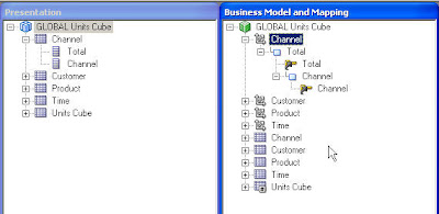
And at first glance, aside from a few updated icons, this version of the Administration tool looks very similar, but the biggest change related to the administration of OLAP data sources (relational or MOLAP) is the ability to map hierarchy objects right through into the presentation layer.
Here is the Metadata generated by the plug-in for the Channel Dimension in both the Business Model and Presentation layers
The new 11g OLAP-style front-end functionality is enabled by adding these hierarchies into the Presentation layer too. This can be achieved by a simple click-and-drag for each hierarchy like the following which is again for the Channel Dimension
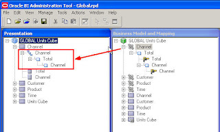
Hopefully, the next release of the plug-in will handle this additional step automatically (and also provide support for value-based hierarchies which were not supported by the front-end in OBIEE 10g) but in the meantime it really is just a simple click-and-drag for each dimension.
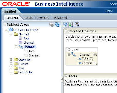
Once all the hierarchies are mapped through into the Presentation Layer, the cube is ready to query. I can log into the OBIEE 11g home page and create a new analysis based upon my Oracle OLAP subject area. The new hierarchies are available for selection when I construct a query
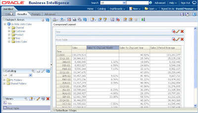
I can then select all of the 'columns' I need for my query and view the results as a pivot table. Here is a really simple example showing Sales by Time. I have also added some calculated measures which have been created inside the AW and derive really useful analytics from the Sales measure. This is a classic reason for using the OLAP Option in the first place - it facilitates the easy creation of calculations that are difficult (or often impossible) to express in SQL. And by having them embedded in the cube, the only thing that the SQL tool (in this case OBIEE) needs to do is select the calculation as a field in a view. How easy is that?!
Once a pivot table with Hierarchy-based columns has been created, this is where the new front-end features really come into play. Some highlights include Calculated Items (derived Dimension members) and a new Selector (which allows dimension selections to be built up as a series of steps based upon add/keep/remove logic):
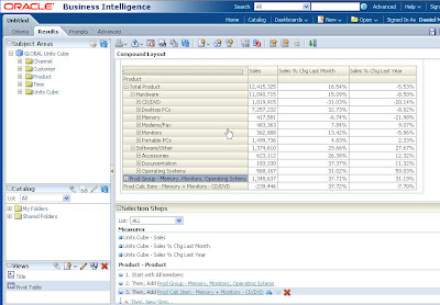
For those familiar with Discoverer OLAP, or Sales Analyzer, Financial Analyzer and Express Objects/Analyzer, these aren't exactly revolutionary features, but combined with all the other great features of the OBIEE suite, this is now a very compelling platform for your Oracle OLAP data.
Finally, I would guess that there are probably thousands of old Oracle Express/OLAP systems that have been waiting for a BI platform like this. If you work on one, what are you waiting for?
***OBIEE 11g can now be downloaded from OTN***
And the fantastic news for Oracle OLAP customers is that OBIEE 11g will work out-of-the-box with Oracle OLAP in almost exactly the same way as OBIEE 10g does - with just one additional configuration step required to enable the new OLAP-style front-end functionality.
Of course, there are other features that are relevant such as the WebLogic application server, and the new security model, but these have already been well blogged elsewhere so the focus of this posting will be Oracle OLAP integration.
To illustrate how easy it is, I will use a trusted old friend as a starting point - the 11g Global sample schema. I have installed this in an Oracle 11.2 database instance, created an Oracle OLAP Analytic Workspace, and then refreshed this AW so that the dimensions and cubes are built.
With an AW in place, the next step is to use the OBIEE plug-in for AWM to generate the metadata required for the OBIEE Server. For those who have not used the plug-in before, check out this excellent demonstration of how it works. While this particular version of the plug-in was originally released to work with OBIEE 10g, and presumably an updated version will be released in due course, it can be used in exactly the same way in OBIEE 11g to import metadata into the Administration tool.

And at first glance, aside from a few updated icons, this version of the Administration tool looks very similar, but the biggest change related to the administration of OLAP data sources (relational or MOLAP) is the ability to map hierarchy objects right through into the presentation layer.
Here is the Metadata generated by the plug-in for the Channel Dimension in both the Business Model and Presentation layers

The new 11g OLAP-style front-end functionality is enabled by adding these hierarchies into the Presentation layer too. This can be achieved by a simple click-and-drag for each hierarchy like the following which is again for the Channel Dimension

Hopefully, the next release of the plug-in will handle this additional step automatically (and also provide support for value-based hierarchies which were not supported by the front-end in OBIEE 10g) but in the meantime it really is just a simple click-and-drag for each dimension.
Once all the hierarchies are mapped through into the Presentation Layer, the cube is ready to query. I can log into the OBIEE 11g home page and create a new analysis based upon my Oracle OLAP subject area. The new hierarchies are available for selection when I construct a query

I can then select all of the 'columns' I need for my query and view the results as a pivot table. Here is a really simple example showing Sales by Time. I have also added some calculated measures which have been created inside the AW and derive really useful analytics from the Sales measure. This is a classic reason for using the OLAP Option in the first place - it facilitates the easy creation of calculations that are difficult (or often impossible) to express in SQL. And by having them embedded in the cube, the only thing that the SQL tool (in this case OBIEE) needs to do is select the calculation as a field in a view. How easy is that?!

Once a pivot table with Hierarchy-based columns has been created, this is where the new front-end features really come into play. Some highlights include Calculated Items (derived Dimension members) and a new Selector (which allows dimension selections to be built up as a series of steps based upon add/keep/remove logic):

For those familiar with Discoverer OLAP, or Sales Analyzer, Financial Analyzer and Express Objects/Analyzer, these aren't exactly revolutionary features, but combined with all the other great features of the OBIEE suite, this is now a very compelling platform for your Oracle OLAP data.
Finally, I would guess that there are probably thousands of old Oracle Express/OLAP systems that have been waiting for a BI platform like this. If you work on one, what are you waiting for?
***OBIEE 11g can now be downloaded from OTN***
Friday, June 18, 2010
Bissantz DeltaMaster - Cool Tool for OLAP
I recently returned from a trip to Germany where visted a Bissantz, a relatively small company in Nürnburg that develops and markets an interesting reporting and data visualization tool named DeltaMaster that works with Oracle OLAP (and other data sources). I was very impressed with this tool. There are few things that I really liked about it:
- It's very good at displaying a lot of information within a single report. One of the ways that it does this is by mixing graphical representations of data with numerical representation (they are very big on something called 'Sparklines'). This makes it very easy to create a single report that includes data on, for example, sales for the current quarter but also provides indications of sales trends and shares.
- The presentation of data is very clean. While the reports themselves are very sophisticated, the developers have done a terrific job of presenting them to users. The presentation tends to be more functional than fluffy, but it's done very well. It is easy on the eyes.
- DeltaMaster goes way beyond basic cross tabs and charts. There are prebuilt reports / analysis templates for rankings, concentration analysis, portfolio analysis, etc. There's quite a few different types of pre-built analysis and I won't try to do justice to them here. See for yourself.
- It works better on OLAP than tables. I'm obviously biased when it comes to this topic, but for the end user this means more analytic power and flexibility.
Below is a concentration analysis report. This is along the lines of a Pareto chart. There are many different types of built-in analysis, but this one looks nice in the confined space of this blog's page.

Here are some links:
The DeltaMaster page at Bissantz: http://www.bissantz.com/products/
A clever blog by Bella, the Bissantz company dog: http://www.bella-consults.com/
Bella, if you happen to find your way to this blog, here's a 'hello' from Henry (the OLAP product manager's dog).

Subscribe to:
Posts (Atom)


